Support:Documents:Examples:FDG with Time-varying Rate Constants
FDG Model with Time-varying Rate Constants
Overview
This example demonstrates how to implement the two-tissue compartment model with extended such that K1 and k2 vary in time.
This models the case where there are physiologic changes during the course of the PET scanning. This might happen if tumors are being treated during scanning.
The standard FDG model was described by Phelps and Huang .
It can also be described by the differential equations:
dCe/dt = K1 Cp - k2 Ce - k3 Ce + k4 Cm
dCm/dt = k3 Ce - k4 Cm
Ce is the tissue concentration of FDG and Cm as the tissue concentration of metabolized FDG (FDG-6-phosphate)
Ce and Cm are interpreted as molar concentrations (Salinas, Muzic and Saidel 2007).
In the standard model. the rate constants K1, k2, k3 and k4 are assumed to be independent of time.
Here we allow K1 and k2 to be linear functions of time:
K1(t) = K10 + a t
k2(t) = k20 + b t
K10 and k20 are the initial (0 superscript) values of the rate constants and a and b are the derivatives (slopes) of the rate constant with respect to time.
To implement the time-varying rate constants, create a MATLAB function in a .m file.
By making the function general, the same function can be used for K1 and k2.
function varargout = kinLinearTime(t, c, ncomp, nsens, pName, pValue, pSensIdx, cm, xtra)
% rate constant varies linearly with time: k = k0 + m*t  where m = dk/dt

K0Name = pName{1};
dkdtName = pName{2};
K0Value = pValue{1};
dkdtValue = pValue{2};
K0SensIndex = pSensIdx{1};
dkdtSensIndex = pSensIdx{2};

if (nargout > 0), % return effective rate constant
    v = K0Value + dkdtValue * t;
    if (v < 0), % don't allow negative values for rate constant
        varargout{1} = 0;
    else
        varargout{1} = v;
    end
    if (nargout > 1),  % return dk/dc
        dkdc = zeros([1 ncomp]);
        varargout{2} = dkdc;
        if (nargout > 2), % return dk/dp
            dkdp = zeros([1 nsens]);
            if (v >= 0),
                dkdp(K0SensIndex) = 1;
                dkdp(dkdtSensIndex) = t;
            end
            varargout{3} = dkdp; % dkdp
            if (nargout > 3),
                ddkdpdc = zeros([ncomp nsens]);
                varargout{4} = ddkdpdc; % ddkdpdc
            end
        end
    end
end
return
This function has a similar pattern to any function one might write to implement customized kinetic rules.
Note the function is called numerous times as the model equations are solved. The value of t (time) takes on values from 0 to the end of the last frame and many values in betweeen - even values that do not correspond to the frame begin and end times.
The first part of the function retrieves values that are automatically sent by COMKAT when it calls this function.
K0Name = pName{1};
dkdtName = pName{2};
K0Value = pValue{1};
dkdtValue = pValue{2};
K0SensIndex = pSensIdx{1};
dkdtSensIndex = pSensIdx{2};
To get COMKAT to call this function, a link (connection between compartments) would be included in the model. For example
cm = addLink(cm, 'LSpecial', 'Cp', 'Ce', 'K1', 'kinLinearTime', {'K10', 'dK1dt'});
When COMKAT calls the custom kinetic function, the last argument of the addLink command ({'K10', 'dK1dt'}) will be passed in as the pName argument.
pValue will be a cell array with the value of pValue{i} set to the value of the parameter named in pName{i}. (Although you could use pxEval to obtain the value of the parameter from pName{i}, it is more efficient for COMKAT to do this internally (only once and cache the result).
pSensIdx will be a cell array with the value of pSensIdx{i} being the position (index) of parameter named in pName{i} in the list of parameters to be estimated.
If the parameter named in pName{i} was not included in an addSensitivity() call, then pSensIdx{i} will be an empty matrix.
The emphasis of the rest of the description of kinLinearTime.m is on the mathematical details.
The first output argument varargout{1} holds the value of the rate constant specified at the current time t. This value is first calculated and stored in the variable v.
v = K0Value + dkdtValue * t
k0 is the rate constant at time zero (t=0) and dkdtValue is the increase in the rate constant per unit time (time-derivative or slope). k0Value and dkdtValue are the MATLAB variables that hold the values of these parameters. The value of v is checked to see if it is negative and, if it is, the value zero is used instead since negative values for rate constants are non-physiologic.
The line
varargout{2} = dkdc;
returns the derivative of the rate constant with respect to all the compartment concentrations (a vector). In this case, the rate constant is not dependent on the concentrations so the derivatives are all zeros.
The lines
dkdp(K0SensIndex) = 1;
dkdp(dkdtSensIndex) = t;
calculate the derivatives of the rate constant with respect to the model parameters k0 (the initial value of the rate constant) and dkdt (the increase in k per unit time). Since a model can have other parameters besides these, the function stores these derivatives in the appropriate element of the derivative vector. Derivatives of this rate constant with respect to all other parameters are zeros.
The line
varargout{4} = ddkdpdc; % ddkdpdc
returns the values of the mixed derivatives (derivative of rate constant with respect to concentrations and with respect to time), which, in this case are all zeros.
The function is stored in kinLinearTime.m in the comkat examples folder.
This function is called to evaluate both K1 and k2.
Implementing the Compartment Model
Create a new model
First define some MATLAB variables for clarity and to facilitate exploring what happens if values are changed
K10 =  0.15;  % K1 = K10 + dK1dt * t
dK1dt = -K10 * 0.5 / 60;  % 50% decrease per 60 minutes
k20 =  0.325; % k2 = k20 + dk2dt * t
dk2dt = -k20 * 0.5 / 60;  % 50% decrease per 60 minutes
k3 = 0.05;
k4 = 0.007;
Next, create a compartment model object and define the parameters within the model object
% create empty compartmentModel object
cm = compartmentModel;

% define the parameters
cm = addParameter(cm, 'K10',   K10);    % 1/min
cm = addParameter(cm, 'k20',   k20);    % 1/min
cm = addParameter(cm, 'k3',    k3);     % 1/min
cm = addParameter(cm, 'k4',    k4);     % 1/min
cm = addParameter(cm, 'dK1dt', dK1dt);  % 1/min/min
cm = addParameter(cm, 'dk2dt', dk2dt);  % 1/min/min

cm = addParameter(cm, 'sa',    1);            % specific activity of injection
cm = addParameter(cm, 'dk',    log(2)/109.8); % F-18 radioactive decay
cm = addParameter(cm, 'PV',    1);            % (none)
Now, define the model compartments. The first two are Ce and Cm as described above and Junk is a "sink" that collects the FDG that is cleared by the venous circulation.
cm = addCompartment(cm, 'Ce');
cm = addCompartment(cm, 'Cm');
cm = addCompartment(cm, 'Junk');
For the plasma concentration time-course of FDG or input function, we'll use the
Feng input
which is an analytic expression. Since piecewise polynomials (linear interpolation, cubic splines, etc...) are widely used in COMKAT and their implementation has been optimized,
here we construct a cubic spline representation of the input function by sampling the Feng input.
x0 = [2 0 500 5 5 -7 -0.1 -0.015];
t = [0:.1:3 3.5 4 4.5 5:1:10 12 15:5:(expDuration+5)];
Cp = fengInput(x0, t);
ppCp = spline(t, Cp);
cm = addInput(cm, 'Cp', 'sa', 'dk', 'ppval', ppCp);  % Cp has units of pmol/ml
The PET scanner measurement is assumed to represent the sum of FDG and FDG-6-Phosphate so the model output is calculated as the sum of the Ce and Cm compartments
Wlist = {...
    'Ce', 'PV';
    'Cm', 'PV'};
Xlist = {};
cm = addOutput(cm, 'PET', Wlist, Xlist);
Next define the scan frames as the start and stop time of each image in the dynamic sequence.
ttt=[ ones(12,1)*10/60; ...  % 10 sec
      ones(10,1)*0.5; ...    %  0.5 min
      ones(10,1)*2;...       %  2 min
      ones(10,1)*5;...       %  5 min
      ones(4,1)*10];         % 10 min
scant=[[0;cumsum(ttt(1:(length(ttt)-1)))] cumsum(ttt)];
cm = set(cm, 'ScanTime', scant);
Note the acquisition begins with 12 frames of 10 sec duration, then has 10 frames of 0.5 minute duration, etc... The cumsum() function calculates the cumulative summation. Thus, the first column of scant holds the scan start times and the second column holds the scan end times. These are expressed in minutes:
scant =

         0    0.1667
    0.1667    0.3333
    0.3333    0.5000
    0.5000    0.6667
    0.6667    0.8333
    0.8333    1.0000
    1.0000    1.1667
    1.1667    1.3333
    1.3333    1.5000
    1.5000    1.6667
    1.6667    1.8333
    1.8333    2.0000
...
Notice thus far the links (arrows) that connect the compartments have not been defined.
This has been delayed since we want to make two models: one will be the standard or reference model with time-invariant rate constants
and one with the time-varying K1 and k2. To make two models, we now make a copy of what we have so far
cmRef = cm;
For the reference model, define the links as time-invariant
% define reference model with time-invariant rate constants
cmRef = addLink(cmRef, 'L',        'Cp', 'Ce',   'K10');
cmRef = addLink(cmRef, 'K',        'Ce', 'Junk', 'k20');
cmRef = addLink(cmRef, 'K',        'Ce', 'Cm',   'k3');
cmRef = addLink(cmRef, 'K',        'Cm', 'Ce',   'k4');
For the fancy model, define the links with the time-varying K1 and k2 rate constants
cm = addLink(cm, 'LSpecial', 'Cp', 'Ce',   'K1', 'kinLinearTime', {'K10', 'dK1dt'});
cm = addLink(cm, 'KSpecial', 'Ce', 'Junk', 'k2', 'kinLinearTime', {'k20', 'dk2dt'});
noting that these make use of the kinLinearTime.m function defined above.
Also, define the time-invariant links
cm = addLink(cm, 'K',        'Ce', 'Cm',   'k3');
cm = addLink(cm, 'K',        'Cm', 'Ce',   'k4');
OK, the models are ready for use. Begin by solving the model to obtain the time-courses of FDG activity that these models predict would be observed in PET images.
[PET, PETIndex] = solve(cm);
[PETRef, PETRefIndex] = solve(cmRef);
Now plot the time-courses. Column 1 of PET (and PETRef) holds the frame start and end times. For convenience, compute the mid-frame time
tmid = (PET(:,1) + PET(:,2)) / 2;
And finally do the plotting
plot(tmid, PET(:,3), 'b', tmid, PETRef(:,3), 'b:');
xlabel('Time (Minutes)');
ylabel('Activity (uCi/ml)');
legend('Time-varying', 'Reference', 'Location', 'SouthEast');
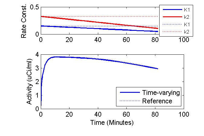
Well, we can get a bit fancy and plot the time-courses of the K1 and k2 rate constants above the model outputs and add other annotations.
clf
axK1k2 = axes('position', [0.2 0.75 0.7 0.2]);
phK = plot(axK1k2, tmid, K10 + dK1dt * tmid, 'b', tmid, k20 + dk2dt * tmid,  'r', ...
             tmid, K10 + 0 * tmid, 'b:',                tmid, k20 + 0 * tmid, 'r:');
set(phK, 'LineWidth', 1.5);
ax = axis; ax(3) = 0; ax(4) = 0.5; axis(ax);
ylabel('Rate Const. (1/min)');
lh = legend('K1', 'k2', 'K1', 'k2', 'Location', 'SouthEast');
set(lh, 'fontsize', 8);

axPET = axes('position', [0.2 0.2 0.7 0.4]);
phPET = plot(axPET, tmid, PET(:,3), 'b', tmid, PETRef(:,3), 'b:');
set(phPET, 'LineWidth', 1.5);
ax = axis; ax(3) = 0; axis(ax);
xlabel('Time (Minutes)');
ylabel('Activity (uCi/ml)');
legend('Time-varying', 'Reference', 'Location', 'SouthEast');
These results are a bit surprising. Why does reducing the both K1 and k2 50% per hour have such a small impact on the model output?
I speculate that the majority of the sensitivity to these parameters occurs when the plasma concentration is high. Also, in this example, the changes in K1 and k2 were proportional such that the ratio was not changing. Why does this matter? Consider the FDG model if there were no phosphorylation (e.g. k3 were zero) so that there was only a single compartment. The differential equation for the compartment would be
dCe/dt = K1 Cp - k2 Ce
At equilibrium, dCe/dt = 0 which implies K1 Cp = k2 Ce or
Ce/Cp = K1 / k2
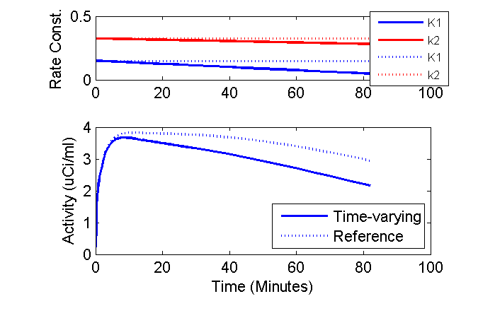
This means, that the example that the equilibrium concentration ratio of tissue to plasma (in absence of phosphorylation) depends only on the ratio K1 / k2. Perhaps in the example once the time gets a bit after the injection and things settle down, the model output is not so sensitive to the individual values K1 and k2 but instead more dependent on their ratio. To test this hypothesis, I can revise the above simulation to consider the case of k2 decreasing 10% per hour so that the ratio K1 / k2 is altered over time. To do this, simply change one line:
Original
dk2dt = -k20 * 0.5 / 60; % 50% decrease per 60 minutes
Revised
dk2dt = -k20 * 0.1 / 60; % 10% decrease per 60 minutes
When the simulation is performed with the new value of k2, the effect of the time-varying rate constants is more evident.
On the other hand, if the rate constants are changing proportionally (as modeled initially), then neglecting the time-variation while fitting data might have a minimal impact.
This is examined next.
Fitting the standard (time-invariant rate constants) model to data with changing physiology
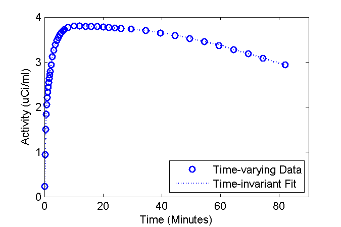
Lets examine the consequences of fitting the standard (time-invariant rate constants) model to data wherein the the physiology (rate constants) are changing. Use the fancy model to create "data" and fit the standard model to that "data".
data = PET(:,3);
cmRef = set(cmRef, 'ExperimentalData', data);
Set the initial guess and lower and upper bounds on the rate constants
pinit = [0.07; 0.1;   0.04;  0.005]; % inital guess
plb =   [0.01; 0.001; 0.001; 0.0001];  % lower bound
pub =   [0.5;  0.5;   0.2;   0.01]; % upper bound
cmRef = addSensitivity(cmRef, 'K10', 'k20', 'k3', 'k4');
Now do the fitting
[pfit, modelFit] = fit(cmRef, pinit, plb, pub);
Plot the fit over the "data"
figure
phFit = plot(tmid, data, 'bo', tmid, modelFit, 'b:');
set(phFit, 'LineWidth', 1.5);
ax = axis; ax(3) = 0; axis(ax);
xlabel('Time (Minutes)');
ylabel('Activity (uCi/ml)');
legend('Time-varying Data', 'Time-invariant Fit', 'Location', 'SouthEast');
Examine estimated values of the rate constants
  Parm.   True (Init->Final)  Est       Est  vs. Init     Units
   K1       0.150 -> 0.041     0.149    -0.4%            1/min
   k2       0.325 -> 0.089     0.324    -0.3%            1/min
   k3       0.050                   0.050    -0.9%            1/min
   k4       0.007                   0.007    1.1%             1/min
   ki        0.020 -> 0.020     0.020    -0.9%            1/min
It turns out that the estimated values are in close agreement with the values of the parameters at time zero (about the time of injection). Thus, in the circumstances simulated here, the model output is pretty insensitive to the significant decreases in K1 and k2.
Get the full example
Note This code for this example can be found in fdgTimeVarying.m in the COMKAT examples folder. That version has a few extra bells and whistles that allow us, for example. to use the FDG model with or without k4.


