Support:Documents:Examples:Estimate Change of Neurotransmitter
Model of Neurotransmitter PET (ntPET)
Overview
The changes of endogenous neurotransmitter by PET scanning after a stimulus have been proved with different approaches. In stead of detecting the increase or decrease of a neurotransmitter, it is important to characterize the temporal change of a neurotransmitter after a stimulus. Morris proposed the new technique (called ntPET) for capturing the dynamic changes of a neurotransmitter after a stimulus and demonstrated the ability of this method to reconstruct the temporal characteristics of an enhance in neurotransmitter concentration.
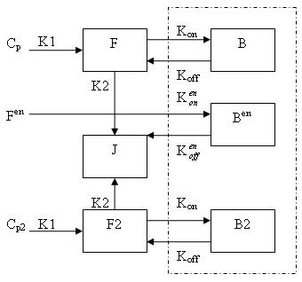
Generally, there are two separate injections of tracer for ntPET: one for the rest condition (without any stimuli) and the other for the activation condition (after a stimulus). Therefore, the model can be described as:
This model can be described by the differential equations:
dF/dt = K1Cp - K2F - Kon[Bmax - B - B2 - Ben]F + koffB
dB/dt = Kon[Bmax - B - B2 - Ben]F - koffB
dF2/dt = K1Cp2 - K2F2 - Kon[Bmax - B - B2 - Ben]F2 + koffB2
dB2/dt = Kon[Bmax - B - B2 - Ben]F2 - koffB2
dBen/dt = Kenon[Bmax - B - B2 - Ben]Fen -kenoffBen
Cp is the plasma concentration of tracer at the first injection (the "rest" condition).
F and B are free (unbound) and bound molar concentrations of tracer after the first injection
Cp2 is the plasma concentration of tracer at the second injection (the "activation" condition).
F2 and B2 are free (unbound) and bound molar concentrations of tracer after the second injection.
Fen and Ben are free and bound molar concentrations of a neurotransmitter released by endogenous ligand after a stimulus.
Bmax is the maximum number of receptors that can be bound by neurotransmitter or tracer.
Bmax - B - B2 - Ben is the concentration of available receptors. This also indicates that binding is saturable.
K1, K2, Kon, Koff, Kenon and Kenoff are rate constants.
Implementing the Compartment Model
Create a new model for ntPET
Step 1. Create the compartemt model
    cm = compartmentModel;

    %Set scan time of the whole scan
    inj2Delay = 240; % min between 1st and 2nd inj
    disp('Define one long study: inj 1 = baseline, inj 2 = activation');
    scantInj1 = [[0:0.1:0.9 1:0.25:1.75 2:0.5:4.5 5:1:59]' [0.1:0.1:1 1.25:0.25:2 2.5:0.5:5 6:1:60]'];
    scantInj2 = scantInj1 + inj2Delay;
    scant = [scantInj1; scantInj2];
    deltaT = scant(:,2) - scant(:,1);
    tmid   = 0.5*(scant(:,1) + scant(:,2));
    cm = set(cm, 'ScanTime', scant);

    %Set parameters of the model
    cm = addParameter(cm, 'PV', 1 );
    cm = addParameter(cm, 'Fv', 0);
    cm = addParameter(cm, 'sa', 1);    % uCi/pmol
    cm = addParameter(cm, 'dk', 0);    % assume data are decay-corrected
    cm = addParameter(cm, 'k1',      0.9);
    cm = addParameter(cm, 'k2',      0.4);
    cm = addParameter(cm, 'kon' ,   0.01);
    cm = addParameter(cm, 'koff',    0.14);
    cm = addParameter(cm, 'k2ref',  0.3);
    cm = addParameter(cm, 'Bmax',  80);
    cm = addParameter(cm, 'konEN', 0.25);
    cm = addParameter(cm, 'koffEN', 25);

    %model for baseline condition:
    cm = addCompartment(cm, 'F');
    cm = addCompartment(cm, 'B',      'Bmax');
    cm = addCompartment(cm, 'Junk');

    %model for activation condition:
    cm = addCompartment(cm, 'F2');
    cm = addCompartment(cm, 'B2',      'Bmax');
    cm = addCompartment(cm, 'B^{EN}', 'Bmax');
Step 2. Set the input function for two injections
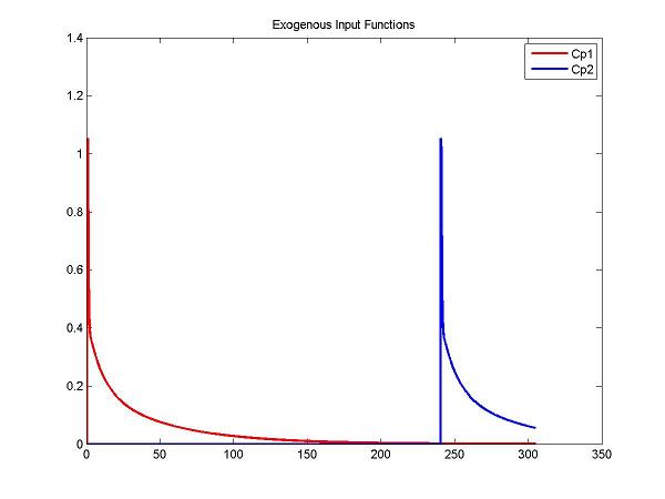
    % Create input functions for two injections
    t = 0:0.05:305; % coverage out to 6+ h
    Cp1Data = fengInput([2 0.5 8.5 0.22 0.2 -4. -0.1 -0.02], t);
    Cp2Data = fengInput([2 inj2Delay+0.5 8.5 0.22 0.2 -4. -0.1 -0.02], t);
    ppCp1 = spline(t, Cp1Data);
    ppCp2 = spline(t, Cp2Data);

    figure; plot(t, ppval(ppCp1, t), 'r', t, ppval(ppCp2,t), 'b', 'LineWidth', 2); title('Exogenous Input Functions'); legend('Cp1', 'Cp2')

    cm = addInput(cm, 'C_p', 'sa', 'dk', 'ppval', ppCp1);
    cm = addInput(cm, 'C_p2', 'sa', 'dk', 'ppval', ppCp2);
Step 3. Create a function described the change of concentrations of the endogenous neurotransmitter. To detect the change, the parameters of the function will be estimated.
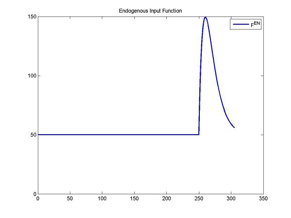
The change of concentrations of the endogenous neurotransmitter after a stimulus is described by a gamma variate function. Fen = Basal + Gamma[t-Delay]Alpha exp(-Beta[t-Delay]). Note: Basal is the concentration of the endogenous neurotransmitter without any stimulus. Gamma, Alpha and Beta control the change of concentrations of the endogenous neurotransmitter. Delay is the delay time.
    DApar = [50 27 1 0.1 240+10]; % = [Basal Gamma Alpha Beta Delay]
    cm = addParameter(cm, 'DA', DApar);
    cm = addInput(cm, 'F^{EN}', 0, 0, 'gammavariate', 'DA'); %DA defined by gamma variate function at activation condition
    figure; plot(t, gammavariate(DApar, t), 'b', 'LineWidth', 2); title('Endogenous Input Function'); legend('F^{en}');
    ax = axis; axis([ax(1) ax(2) 0 ax(4)]); % ensure minimum y-axis value is zero
The endogenous input function is implemented as (create the below function and put in in a file called gammavariate.m):
function [y, grad] = gammavariate(p,t)
% parameters [p(1) p(2) p(3) p(4) p(5)] = [Basal G alpha beta delay]
    y = p(1).*ones(size(t));
    idx = find(t >= p(5));
    dt  = t(idx) - p(5);

    y(idx) = p(1) + p(2)*(dt.^p(3)).*exp(-p(4).*dt);

    if nargout > 1,
        grad = zeros(length(t), 5);
        grad(:,1)=ones(size(t));

        if ~isempty(idx),
            grad(idx,2) = (dt).^p(3).*exp(-p(4).*(dt));
            grad(idx,3) = p(2).*(dt).^p(3).*log(dt).*exp(-p(4).*(dt));
            grad(idx,4) = -p(2).*(dt).^(p(3)+1).*exp(-p(4).*(dt));
            grad(idx,5) = -p(2)*p(3)*(dt).^(p(3)-1).*exp(-p(4).*(dt)) + p(2)*p(4)*(dt).^p(3).*exp(-p(4).*(dt)); %dy/ddelay
        end
    end
return
Step 4. Set link between each compartment and add output.
    %links/output for baseline condition:
    cm = addLink(cm, 'L',  'C_p',     'F',      'k1');
    cm = addLink(cm, 'K',  'F',       'Junk',   'k2');
    cm = addLink(cm, 'K2', 'F',       'B',      'kon');
    cm = addLink(cm, 'K',  'B',       'F',      'koff');

    disp('Output is sum of radioactivity in free and bound compartments')
    WList = {...
          'F', 'PV';
          'F2', 'PV';
          'B', 'PV';
          'B2', 'PV'};
    XList = {};
    cm = addOutput(cm, 'PET Scan', WList, XList);

    %links/output for activation condition:
    cm = addLink(cm, 'L',  'C_p2',     'F2',      'k1');
    cm = addLink(cm, 'K',  'F2',       'Junk',    'k2');
    cm = addLink(cm, 'K2', 'F2',       'B2',      'kon');
    cm = addLink(cm, 'L2', 'F^{EN}',  'B^{EN}', 'konEN');
    cm = addLink(cm, 'K',  'B2',       'F2',      'koff');
    cm = addLink(cm, 'K',  'B^{EN}',  'Junk',    'koffEN');
    cm = addSensitivity(cm, 'DA', 'k1', 'k2', 'kon', 'koff', 'k2ref');  % set desired 'estimated parameters'
Step 5. Solve the model and generate the output
     disp('Properly handle the initial conditions assuming no exogenous ligand initially')
     IC.time = 0;
     Kd = pxEval(cm, 'koffEN') / pxEval(cm, 'konEN');
     Bmax = pxEval(cm, 'Bmax');
     FEN = gammavariate(DApar, 0);
     compNames = get(cm, 'CompartmentName');
     sensNames = get(cm, 'SensitivityName');
     idxBEN = strmatch('B^{EN}', compNames);
     idxBasal = strmatch('DA', sensNames); % DA is a vector-valued parameter and Basal is its 1st element
     ncomp = get(cm, 'NumberCompartments');

     %initialize cell array, if matrix is used then solver error is thrown sometimes
     IC.compartment =cell(ncomp,1);
     for j = 1:ncomp
        IC.compartment{j} = 0;
     end
     IC.compartment{strmatch('B^{EN}', compNames, 'exact')} = Bmax * FEN / (Kd + FEN);

     IC.compartmentSensitivity = zeros([length(compNames) length(sensNames)]);
     IC.compartmentSensitivity(idxBEN, idxBasal) = Bmax*Kd / ((Kd + FEN)^2); %dBEN/dBasal calculated correctly now
     cm = set(cm, 'InitialConditions', IC);

    [PET, PETIndex, Output, OutputIndex] = solve(cm);

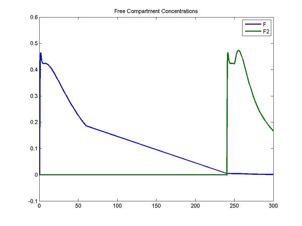
    disp('Plot some compartment concentrations to examine model behavior');
    figure; idx = [3 6]; plot(Output(:,1), Output(:, idx), 'LineWidth', 2); legend(OutputIndex(idx)); title('Free Compartment Concentrations');
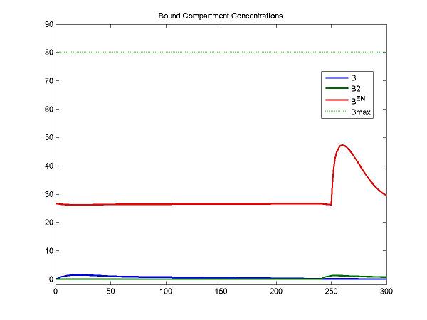
    figure; idx = [4 7 8]; plot(Output(:,1), Output(:, idx), [0 Output(end,1)],  [Bmax Bmax], 'g:', 'LineWidth', 2); legend(OutputIndex(idx), 'Bmax'); title('Bound
    Compartment Concentrations');
