Support:Documents:COMKAT Examples
Example 1: Estimate Input Parameters, Rate Constants Known
Here we assume that the input function has the form
Cp = (p1t - p2 - p3) exp(-p4t) + p2 exp(-p5t) + p3 exp(-p6t)
where Cp is the plasma concentration of 18FDG, pi are the input function parameters to be estimated, and t is time. (This form comes from Feng, Huang, Wang. "Models for Computer simulation Studies of Input Functions for Tracer Kinetic Modeling with Positron Emission Tomography", International Journal of Biomedical Computing, 32(2):95-110, March 1993.)
Step 1 To set this up in MATLAB for simulation, create the following function and put it in a file called refCp.m:
function [fval, jac] = refCp(p, t)
 if (nargout > 0),
       t = t(:);  % make it a column vector
       fval = (p(1)*t - p(2) - p(3)) .* exp(-p(4)*t) + p(2) * exp(-p(5)*t) + p(3) * exp(-p(6)*t);
       if (nargout > 1),
           jac = [t .* exp(-p(4)*t) ...
                  -exp(-p(4)*t) + exp(-p(5)*t) ...
                  -exp(-p(4)*t) + exp(-p(6)*t) ...
                  -t .* (p(1)*t - p(2) - p(3)) .* exp(-p(4)*t) ...
                  -t * p(2) .* exp(-p(5)*t) ...
                  -t * p(3) .* exp(-p(6)*t)];
       end
   end
return
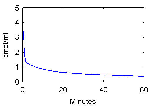
This function can be used to plot an example input curve using these commands
   t=0:.1:60;
   pin = [28 0.75 0.70 4.134 0.1191 0.01043];
   plot(t,refCp(pin,t))
   set(gca,'FontSize',6);
   axis([0 60 0 5]);
   xlabel('Minutes');
   ylabel('pmol/ml');
Note that he above function, refCp.m not only calculates values Cp, it also optionally calculates values for the derivative of Cp with respect to parameter vector p. These will be needed later since to fit the input function, it is important to quantify how changes in values of p will effects Cp values which, in turn, effect model-predicted tissue concentration reflected in voxels or regions of interest.
Step 2 Create an FDG model
   cm = compartmentModel;

   %        k1     k2      k3     k4
   ktrue=[0.1020 0.1300 0.0620 0.0068];

   % define the parameters
   cm = addParameter(cm, 'k1',    ktrue(1));     % 1/min
   cm = addParameter(cm, 'k2',    ktrue(2));     % 1/min
   cm = addParameter(cm, 'k3',    ktrue(3));     % ml/(pmol*min)
   cm = addParameter(cm, 'k4',    ktrue(4));     % 1/min
   cm = addParameter(cm, 'sa',    75);           % specific activity of injection, kBq/pmol
   cm = addParameter(cm, 'dk',    log(2)/109.8); % radioactive decay
   cm = addParameter(cm, 'PV',    1);            % (none)

   % define input function parameter vector
   cm = addParameter(cm, 'pin', [28; 0.75; 0.70; 4.134; 0.1191; 0.01043]);

   % define compartments
   cm = addCompartment(cm, 'Ce', );
   cm = addCompartment(cm, 'Cm', );
   cm = addCompartment(cm, 'Junk', );

   % define plasma input function
   % specifying function as refCp with parameters pin
   cm = addInput(cm, 'Cp', 'sa', 'dk', 'refCp', 'pin'); % plamsa pmol/ml

   % connect inputs and compartments
   cm = addLink(cm, 'L', 'Cp', 'Ce', 'k1');
   cm = addLink(cm, 'K', 'Ce', 'Junk', 'k2');
   cm = addLink(cm, 'K', 'Ce', 'Cm', 'k3');
   cm = addLink(cm, 'K', 'Cm', 'Ce', 'k4');

   % specify scan begin and end times
   ttt=[ ones(6,1)*5/60; ...    %  6 frames x  5   sec
         ones(2,1)*15/60; ...   %  2 frames x 15   sec
         ones(6,1)*0.5;...      %  6 frames x  0.5 min
         ones(3,1)*2;...        %  3 frames x  2   min
         ones(2,1)*5;...        %  2 frames x  5   min
         ones(10,1)*10];        % 10 frames x 10   min
   scant = [[0;cumsum(ttt(1:(length(ttt)-1)))] cumsum(ttt)];
   cm = set(cm, 'ScanTime', scant);

   % define an output which is sum of Ce and Cm adjusted to account
   % for partial volume (PV).  Ignore vascular activity.
   Wlist = {...
       'Ce', 'PV';
       'Cm', 'PV'};
   Xlist = {};
   cm = addOutput(cm, 'PET', Wlist, Xlist);

   % solve model and generate example output
   [PET, PETindex]=solve(cm);
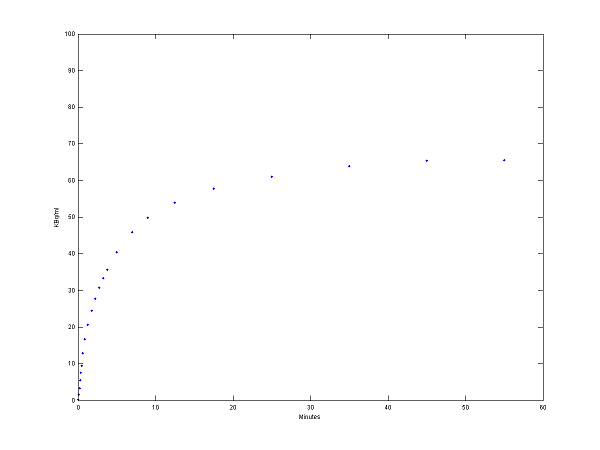
   plot(0.5*(PET(:,1)+PET(:,2)),PET(:,3), '.');
   set(gca,'FontSize',6);
   axis([0 60 0 100])
   xlabel('Minutes');
   ylabel('KBq/ml');
Step 3 Use model output as perfect "data"
data = PET(:,3);
Step 4 Fit the "data"
   % tell model abbout data to be fit
   cm = set(cm, 'ExperimentalData', data);

   % specify parameters to be adjusted in fitting
   cm = addSensitivity(cm, 'pin');

   % set parameter values initial guess, lower and upper bounds
   pinit = [ 10; 0.4;  0.4;  3;  0.05; 0.01];
   plb =   [ 10; 0.1;  0.1;  1;  0.05; 0.001];
   pub =   [100; 2. ;  2. ; 10;  1.  ; 0.05];

   % actually do the fitting
   pfit = fit(cm, pinit, plb, pub);
Values of parameter pfit estimates are [28.0167; 0.7652; 0.7059; 4.1586; 0.1257; 0.0105] and are reasonably close to the true values (pxEval(cm, 'pin')) [28; 0.75; 0.70; 4.134; 0.1191; 0.01043]
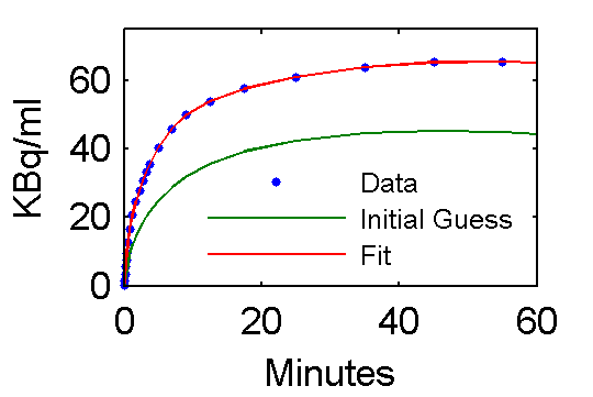
Step 5 Examine model outputs for "data", initial guess, and fit
   PETfit = solve(set(cm, 'ParameterValue', 'pin', pfit));
   PETinit = solve(set(cm, 'ParameterValue', 'pin', pinit));
   t = 0.5*(PET(:,1)+PET(:,2));
   plot(t,data,'.', t, PETinit(:,3), t, PETfit(:,3));
   set(gca,'FontSize',8);
   axis([0 60 0 75])
   xlabel('Minutes');
   ylabel('KBq/ml');
   ah=legend('Data', 'Initial Guess', 'Fit','Location','SouthEast');
   set(ah,'FontSize',6,'Box','off');
Simplified reference tissue method
This example demonstrates a COMKAT implementation of the simplified reference tissue model (SRTM) described by Lammertsma and Hume [Neuroimage. 4(3 Pt 1), 153-158 (1996)]. By simultaneously analyzing time-activity curves from areas with and without receptors, the SRTM provides a means to estimate the binding potential which is an index of receptor concentration and ligand affinity.
Background
Input functions are a fundamental component of pharmacokinetic modeling. They describe the time-course of (radio)pharmaceutical which is accessible to the extravascular space. In PET receptor studies the arterial plasma concentration of a ligand is taken as the input function. As there is desire to obviate blood sampling, the SRTM is a popular method used to analyze ligand-receptor data.
The typical model equations used for a region containing receptors include state equations for free (F) and bound (B) ligand:
| dF/dt = k1 Cp – (k2+k3)F + k4 B | Eq 1 |
| dB/dt = k3 F – k4 B | Eq 2 |
where Cp is the arterial plasma input function and tracer conditions are assumed (B << Bmax) so that k3 = kon (Bmax – B) ≈ kon Bmax.
In a region devoid of receptors, k3 (and therefore B) is zero so Eq 1 may be simplified. Denoting this region as the reference region, or rr, the equation is
| dFrr/dt = k1 Cp – k2rr Frr | Eq 3 |
This may be rearranged to obtain an expression for the plasma input
| Cp = Cpn / k1rr | Eq 4 |
where
| Cpn = (dFrr/dt + k2rr Frr) | Eq 5 |
is the normalized plasma input function.
This expression (Eq 4) for Cp may be substituted into the equations for regions that have receptors, aka, target tissue which we denote as tt
| dFtt/dt = (k1tt/k1rr) Cpn – (k2tt+k3tt)Ftt + k4tt Btt | Eq 6 |
| dBtt/dt = k3tt Ftt – k4tt Btt | Eq 7 |
Data from target tissue and from reference regions could be, in theory, simultaneously fit using the model embodied in Eq. 4 to 6. In practice there is often an issue of identifiability. Hence, assumptions are made to reduce the number of parameters to estimate. One assumption is that the equilibrium concentration ratio between plasma and tissue free space is the same in the reference region and target tissue:
| k1tt/ k2tt= k1rr /k2rr | Eq 8 |
this implies
| k1tt/k1rr = k2tt/k2rr | Eq 9 |
and this ratio may be denoted by R1
| R1 = k1tt/k1rr = k2tt/k2rr | Eq 10 |
Making the substitution into Eq 6 we obtain
| dFtt/dt = R1 Cpn – (k2tt+k3tt)Ftt + k4tt Btt | Eq 11 |
This equation could be solved simultaneously with Eq. 7 to obtain time-courses of free and bound radioligand. Analytic solutions derived for more general conditions (Eq 1 and 2) are given in the appendix in the document thad describes validation of the COMKAT implementation of the FDG model. Solutions for Ftt and B tt would then be summed to obtain the total concentration in the target tissue which is the quantity measured in an imaging study
| Ct = Ftt+Btt | Eq 12 |
In general, the solution Ctt is a weighted sum of two exponential terms. For ligands in which the association and dissociation of ligand from the receptor is much faster than the transport of ligand between the vascular and extravascular space, two exponentials are not evident from the data. That is, a single exponential model adequaltey describes the data because the two compartments exchange so quickly that they look like a single compartment. (Mathematically one of the eigenvalues or exponential coefficients is very large in magnitude.) The differential equation for such a single-exponential model is
| dCtt /dt = k1tt Cp –k2att C tt | Eq 13 |
where k2att is the the apparent k2tt and is related to the the other parameters as
| k2att = k2tt /(1+BP) | Eq 14 |
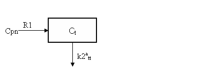
where BP = k3tt/k4tt is the binding potential. Expressing the input in terms of Cpn, this is equivalent to the one-tissue compartment model depicted below
COMKAT Implementation
comkat\examples\dasbSRTM.m
Step 1 To set this up in MATLAB, create an input function that implements Eq. 5 [Cpn = (dFrr/dt + k2rr Frr)]. In this k2rr is a parameter to estimate amd Frris taken as experimentally measured reference region concentration. To obtain Frr at arbitrary times requires interpolation. For this a smoothing spline is used. Its piecewise-polynomial coefficients are easily obtained
ppCref = csaps(tref, Cref, 0.01);
where tref and Cref are the sample times and concentrations from the reference region. With Frr expressed in this form, the polynomials may be analytically differentiated once to obtain the piecewise polynomial coefficients of dFrr/dt
ppdCrefdt = fnder(ppCref, 1);
The input Cpn may be evaluated as Cpn(t) = k2rr x ppval(ppCref. t) + ppval(ppdCrefdt.t) with the complete function given in comkat\examples\refInput.m
function [Cpn, dCpndk2ref] = refInput(k2ref, t, pxtra)
  ppCref = pxtra{1};
  ppdCrefdt = pxtra{2};
  if (nargout > 0),
    Cpn = k2ref * ppval(ppCref, t) + ppval(ppdCrefdt,t);
    idx = find(Cpn < 0);
    Cpn(idx) = 0;
    if (nargout > 1),
      dCpndk2ref = ppval(ppCref, t);
      dCpndk2ref(idx) = 0;
    end
  end
return
For the sake of estimating the value of k2rr, this function must provide the derivative of Cpn with respect to k2rr when two output arguments are requested.
This input function is included in the compartment model by using these commands
sa = 1; % specific activity
dk = 0; % decay constant (=0 since data are decay corrected)
xparm = { ppCref, ppdCrefdt };
cm = addInput(cm, 'Cpn', sa, dk, 'refInput', 'k2ref', xparm);
Step 2 Create a model. To simultaneously fit three regions – midrbain, amygdala, and thalamus – create a model that has the compartments and links depicted as shown. Three Region Model
The commands are
% specify compartments
cm = addCompartment(cm, 'Cmid');
cm = addCompartment(cm, 'Camy');
cm = addCompartment(cm, 'Ctha');
cm = addCompartment(cm, 'Sink'); % comkat requires closed system

% specify links
cm = addLink(cm, 'L', 'Cpn',  'Cmid',  'R1mid');  % connect input to
cm = addLink(cm, 'K', 'Cmid', 'Sink',  'k2ppmid');

cm = addLink(cm, 'L', 'Cpn',  'Camy',  'R1amy');
cm = addLink(cm, 'K', 'Camy', 'Sink',  'k2ppamy');

cm = addLink(cm, 'L', 'Cpn',  'Ctha',  'R1tha');
cm = addLink(cm, 'K', 'Ctha', 'Sink',  'k2pptha');

% specify outputs (neglect vascular contrib)
% for simultaneously fitting target tissues
cm = addOutput(cm, 'Mid', {'Cmid', 'PV'}, { } );
cm = addOutput(cm, 'Amy', {'Camy', 'PV'}, { } );
cm = addOutput(cm, 'Tha', {'Ctha', 'PV'}, { } );

% specify parameters and values
cm = addParameter(cm, 'PV',    1);
cm = addParameter(cm, 'k2ref', 0.05);

cm = addParameter(cm, 'R1mid', 0.8);
cm = addParameter(cm, 'R1amy', 1.0);
cm = addParameter(cm, 'R1tha', 1.2);

cm = addParameter(cm, 'BPmid', 0.5);
cm = addParameter(cm, 'BPamy', 1.0);
cm = addParameter(cm, 'BPtha', 1.5);

cm = addParameter(cm, 'k2ppmid', 'k2ref*R1mid/(1+BPmid)');
cm = addParameter(cm, 'k2ppamy', 'k2ref*R1amy/(1+BPamy)');
cm = addParameter(cm, 'k2pptha', 'k2ref*R1tha/(1+BPtha)');
The rest of the details are quite straightforward and are all contained in the example file comkat\examples\dasbSRTM.m. The only thing slightly unusual is that multiple time-activity curves must be specified so they can be simultaneously fit. To do this, just use
cm = set(cm, 'ExperimentalData', PETdata(:, [1 2 3]));
where columns [1 2 3] contain 'Mid', 'Amy', and 'Tha' data [the same order as the adddOutput() commands] and the rows of PETdata correspond to different frames.
Glucose minimal model
This example shows a COMKAT implementation of the glucose minimal model (GMM) which describes the interaction between glucose and insulin in vivo. One model compartment represents interstitial insulin concentration which is denoted by X. Another model compartment represents plasma glucose concentration which is denoted by G. This model was presented in Bergman RN, Ider YZ, Bowden CR, Cobelli C. "Quantitative estimation of insulin sensitivity," Am. J. Physiol., vol. 236, no. 6, pp. E667-E677, June 1979.
Background
Of particular note is that this model has an unusual nonlinear kinetic rule that is different from the nonlinear receptor-ligand and enzyme-substrate kinetic rules. Implementing this GMM in COMKAT required definition of a custom kinetic rule as this example demonstrates. This example also demonstrates COMKAT's ability to solve sensitivity functions (and hence estimate the value of) a parameter which is an initial condition to the differential equations.
Model Equations
dX/dt = -p2 X + p3(I - Ib)
dG/dt = -GX + p1(Gb - G)
with initial conditions X = 0, G = p4 at time zero.
X is interstitial insulin concentration. G is plasma glucose concentration. I is plasma insulin concentration. Ib and Gb are basal insulin and glucose concentrations. p1 to p4 are model mathematical parameters. They are related to the physiologically meaningful parameters as follows
- Glucose effectiveness, SG = p1, a measure of the fractional ability of glucose to enhance its own clearance independent of insulin
- Insulin sensitivity, SI = p3/p2, a measure of the dependence of fractional glucose disposal on changes of plasma insulin
- Initial glucose concentration, G(0) = p4
COMKAT Implementation
To implement the unusual non-linear kinetics present for glucose in COMKAT, the glucose state equation is rearranged to obtain
dG/dt = -G(X + p1) + p1Gb
and the expression (X + p1) is considered as a rate "constant".
Otherwise, the COMKAT implementation is straighforward and the diagram is depicted below.
Model Diagram
Since COMKAT requires a closed system, two junk or sink compartments were created (J1 and J2) so that the efflux from X and G would have a destination.
The complete example is given in comkat\examples\comkatGMM.m.
As the glucose minimal model is used to analze blood sample data (and not an image-based data set) for which people usually assume blood samples represent instantaneous (and not the time-averaged) concentration, this example only considers compartment concentrations (and not the output equations). Accordingly, the plots here are based on solutions to the compartment concentrations which are placed in comp when the model is solved using this command:
[out, outIndex, comp, compIndex] = solve(cm);
Plots of G and X versus time are shown here:
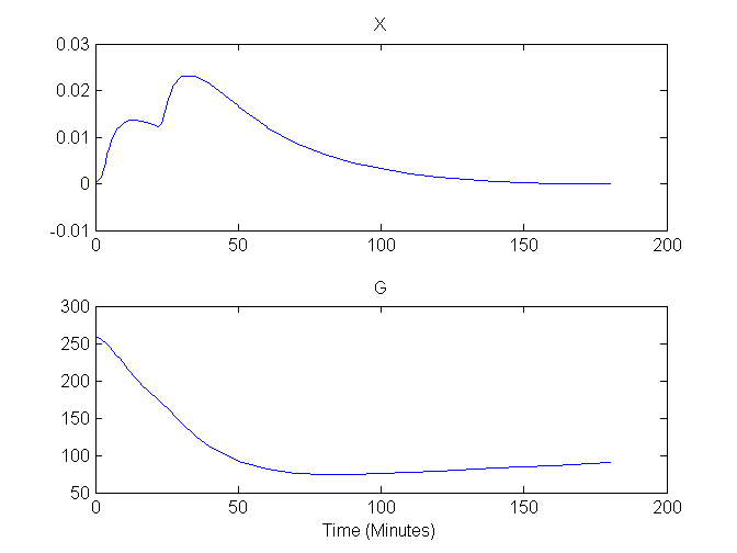
Compartment Concentrations and plots of compartment sensitivity functions, derivatives of X and G with respect to the model parameters, are shown below
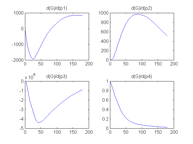
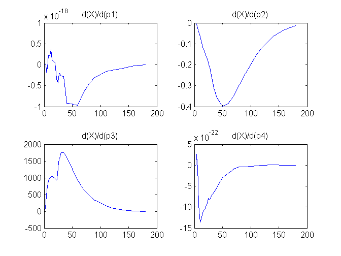
Notice that the plots of the sensitivity functions suggest variable X is independent of parameters p1 and p4 as d(X)/d(p1) and d(X)/d(p4) are zero (within the numerical precision). This is expected because a) the state equation for X has neither p1 nor p4 terms and b) G, which appears on the right hand side of the state equation for X, is independent of p1 and p4.
NOTE: GMM is also implemented as part of the validation suite wherein solutions to a COMKAT and an independent implementation are compared.
Enzyme-substrate (Michaelis-Menten) kinetics
This example demonstrates COMKAT implementation of enzyme substrate (Michaelis Menten) kinetics. This is a type of kinetic rule in which reaction velocity is saturable. As such, this example demonstrates use of a user-specified custom kinetic rule.
Background
Enzymes act as catalysts speeding up reactions wherein a substrate is converted to product without the enzymes themselves being consumed in the process. When the amount of enzyme is much less than the amount of substrate, the effective rate constant k is not actually a constant but rather depends on the substrate concentration
k = Vmax / (Km + [S])
This relationship is described and derived here and requires a couple of approximations.
A COMKAT implementaion of a model that includes such kinetics is given below. The complete model that avoids the two approximations could also be implemented in COMKAT and will be left as an exercise for the student ;-).
COMKAT Implementation
Model figure
File:ModelFigure.png This example demonstrates how to implement in COMKAT a model that incorporates the Enzyme-Substrate kinetics using a rate "constant" with a value that depends on substrate concentration. In the interest of simplicity, this example only includes only two compartments and one link. Of course more complicated models could be constructed, yet this example is sufficent to demonstrate the concept.
Step 1 To set this up in MATLAB for simulation, create the following function that defines the rate "constant" for this kinetic rule:
function varargout = kinMM(t, c, ncomp, nsens, pName, pValue, pSensIdx, cm, xtra)
  % Michaelis Menten kinetics
  % flux = C * Vmax/(Km + C) so that effective
  % rate constant k = Vmax/(Km + C)
  VmName = pName{1};
  KmName = pName{2};
  VmValue = pValue{1};
  KmValue = pValue{2};
  VmSensIndex = pSensIdx{1};
  KmSensIndex = pSensIdx{2};
  substrateCompartmentIndex = xtra{1};
  if (nargout > 0), % return effective rate constant
    varargout{1} = VmValue / (KmValue + c(substrateCompartmentIndex));
    if (nargout > 1),  % return dk/dc
        dkdc = zeros([1 ncomp]);
        dkdc(substrateCompartmentIndex) = VmValue / (KmValue + c(substrateCompartmentIndex)).^2;
        varargout{2} = dkdc;
        if (nargout > 2), % return dk/dp
            dkdp = zeros([1 nsens]);
            dkdp(VmSensIndex) = 1 / (KmValue + c(substrateCompartmentIndex));
            dkdp(KmSensIndex) = VmValue / (KmValue + c(substrateCompartmentIndex)).^2;
            varargout{3} = dkdp; % dkdp
        end
    end
  end;
  return;
As for all custom kinetic rules, this function must adhere to the call signature with 8 (or optionally 9) input arguments whether or not all inputs are used. The inputs are
t 	  	    time
c 	  	   Vector of compartment concentrations
ncomp 	       Number of compartments in the model
nsens 	  	Number of parameters for which sensitivity functions are requested (e.g. the number of parameters being estimated_
pName 	      Cell array of character strings. E.g. pName{1} = 'Vm', pName{2} = 'Km'
pValue 	Cell array with pValue{i} being the value of pName{i}
pSensIdx     Cell array containing indicies (locations) of pName{i} in the sensitivityName [addSensitivity()] parameters.
cm 	  	The compartmentModel object
xtra 	  	Any extra information that the user would like to be passed to the function [this input is optional]
The kinMM function is bit complicated because it was written to be general. The compartments that are the source and destination of the link are not hardcoded but rather determined based on the value of the input arguments. Likewise, the names of the parameters that are used to identify what are traditionally described as Km and Vmax are also be specified. Not only does this allow a user call the parameter whatever suits his or her fancy (e.g. the Km value could be specified by a parameter called 'Fred'), it also facilitates models with more than one link that is described by enzyme-substrate kinetics. Writing the function to be general in this fashion obviates having to write a separate kinetic rule function for each model. (The newest verion of the function above is available in comkat\examples\kinMM.m).
One thing to notice about the function above is that the line
varargout{1} = VmValue / (KmValue + c(substrateCompartmentIndex));
corresponds to the equation given in Background.The substrate concentration [S] is taken as the concentration in the source compartment.
Another thing to notice is that the function should return 0, 1 or more values depending nargout. The first return value would be the value of the rate "constant". The second return value would be the derivaive of the rate constant with respect to the concentration vector. The third return value would be the derivative of the rate constant with respect to the sensitivity parameters. These latter two are used in calculating the derivative of model output with respective to sensitivity parameters which is important in data fitting.
Step 2 Create the model.
conc = 10; % initial substrate concentration

cm = compartmentModel;
cm = addCompartment(cm, 'Substrate');
cm = addCompartment(cm, 'Product');
cm = addParameter(cm, 'Km', 10);
cm = addParameter(cm, 'Vm', 0.5);
cm = addParameter(cm, 'dk', 0); % specific activity
cm = addParameter(cm, 'sa', 1); % decay constant


% define the time
tmin = 0;
tmax = 120;
t = [0:1:tmax]';
scanTime = [t t+0.01];
cm = set(cm, 'ScanTime', scanTime);

% details needed for MM kinetics link
substrateCompartmentIndex = { 1 };
pName = {'Vm', 'Km'};           % Vm and Vm parameter names
cm = addLink(cm, 'KSpecial', 'Substrate', 'Product', 'Kmm', 'kinMM', pName, substrateCompartmentIndex);

% set initial concentration and TIME
IC.time = 0;
IC.compartment = [conc; 0];  % all substrate, no product
cm = set(cm, 'InitialConditions', IC);

% run the model
[cAvg, cAvgIdx, c1, cIdx]  = solve(cm);


% repeat experiment with more substrate
IC.compartment = [4*conc; 0];  % all substrate, no product
cm = set(cm, 'InitialConditions', IC);
[cAvg, cAvgIdx, c2, cIdx]  = solve(cm);

% plot results
plot(c1(:,1), c1(:,[2 3]), c2(:,1), c2(:,[2 3]));
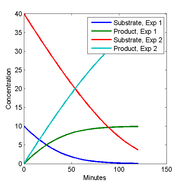
legend('Substrate, Exp 1', 'Product, Exp 1', 'Substrate, Exp 2', 'Product, Exp 2')
The plot looks like this.
A slightly more elaborate version of this example can be found in comkat\examples\tutorialMichaelisMenten.m
