3D Reslicing using COMKAT image tool (basic)

Reslicing 3D image volume using COMKAT image tool (basic)

Overview

Reslicing a 3D (or 3D vs time) image dataset can be accomplished using various components of COMKAT including the function sliceVolume() which is a method of ImageVolumeData. This example explains how to create a 2D image by sampling (slicing) from a volume at a position, plane orientation, and magnification specified by the user. The approach is to load the image volume dataset into an instance of an ImageVolumeData (abbreviated IVD) object and to use the sliceVolume() method.

Background

sliceVolume() is a mex-file written in c with an interface to MATLAB that makes the operation particularly efficient. COMKATImageTool uses sliceVolume() and you can use it too.

Approach I. Demonstrate the method for coordinate transformations

Create an instance of an IVD object and load it with an image volume.

  ivd = ImageVolumeData(); % create an instance of an ImageVolumeData object
  ivd = read_DICOM(ivd, pathName, fileName); % load volume into an instance of IVD object;

Create lists of indices of all pixels in the 2D slice (rectangular grid) that we are creating.

  [i, j] = meshgrid(0 : Nc-1, 0 : Nr-1); % i and j will be 2D arrays, meshgrid is a function built into MATLAB
  ij = [i(:)' ; j(:)'];  % make matrix, each column corresponding to a single pixel in the slice we are creating

The first and second rows of ij are the indices corresponding to column and row indices of all voxels in the desired slice. So the dimension of ij is 3 x ( # of desired voxels ).

Note: the first column of ij could be [ 0 ; 0 ] ; the second column could be [ 0 ; 1 ] , etc.

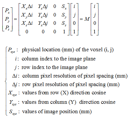
Then, we need to compute the physical x,y,z locations, in mm, from desired voxel indices according to the DICOM coordinate system ref [1] p. 275. According the ref, the coordinate transformation matrix, M, is listed as follows:

The transformation matrix can be further separated into three parts.

Once we set the transformation matrix (or the orientation, pixel spacing, and image position matrices), we can use the transformation matrix to calculate the physical (mm) locations of each voxel in the desired slice.

  xyz = M * ij; 
      or
  xyz = M_orientation * M_spacing * ij + M_position  ; 
  
  *  xyz is a matrix consisted of three rows the physical x, y, and z location (m) of all the desired voxels. The dimension of xyz is 3 x ( # of desired voxels ).

These xyz locations are the same as those in the image volume that is being sliced to make the 2D image. From these xyz locations, we find the corresponding 3D indices, (u,v,w), in the volume. This uses the transformation matrix for the volume, Mhat, that relates the indices to the xyz physical location. This is analogous to M used for the desired slice but here the pixel spacing, orientation, and position indicate how the volume data are stored.

The spatial mapping between the indices in the original image volume (uvw) and xyz can be described as

  xyz = Mhat * uvw;

Therefore, Mhat is the matrix mapping uvw to its physical location (mm) and can be separated into three parts, M'_orientation, M'_spacing, and M'_position, as the transformation M.

Note: M'_orientation, M'_spacing, and M'_position are the mapping matrices between uvw and xyz which are different from the mapping matrices between ij and xyz.

The indices of the desired slice can be calculated by performing the inverse mapping.

  uvw =  inv( Mhat ) * xyz;    
      or
  uvw = inv( M'_spacing ) * inv( M'_orientation ) * (xyz - M'_position ) ; 
  
  * uvw is the matrices consisted of the indices in the domain of the original volume and is consisted of three rows corresponding to row, column, and plane indices of the original volume data.
     The dimension of uvw is identical of that of xyz.

In order to use sliceVolume() to do the interpolation, we need to separate uvw into the components

    u = ( row indices in the domain of original of volume data );
    v = ( column indices in the domain of original of volume data );
   w = ( plane indices in the domain of original of volume data );
  
   *Note: the u, v, w are the first, second, and third rows of uvw.

Before doing interpolation, we have to set a unscaled raw background value of images, rawbackgroundPixelValue. The value is used for the interpolation when it is nothing there for calculating the interpolation value.

In gerneral, rawbackgroundPixelValue = (scaled_pixel_value - rescale_intercept) / (rescale_slope) ;

For PET images, the scaled background value is usually zero.

==>    rawbackgroundPixelValue  = ( 0 - rescale_intercept) / rescale_slope ;

So rawbackgroundPixelValue can be calculated as follows:

  s = get( ivd, 'VolumeFrameBufferScaleFactor');           % rescale_slope
  o = get( ivd, 'VolumeFrameBufferRescaleIntercept');  % rescale_intercept
  
  rawbackgroundPixelValue  = - o / s;

Finally, we use sliceVolume() to interpolate the desired slice

  slice = sliceVolume(idv, v, u, w, rawbackgroundPixelValue , 'linear');

Approach II. Use coordinateGen() to do the coordinate transformation

This should create same result as approach I but require fewer lines of coding since coordinateGen() does most things that are needed.

Read the image volume into an ImageVolumeData object

  ivd = ( read data into IVD);

Use coordinateGen() to generate uvw

  [u, v, w] = coordinateGen(ivd, Nc, Nr, pixelSpacing, planePos, orientation); % Input the desired pixelSpacing, planePos and orientation matrices

Use sliceVolume() to interpolate

  slice = sliceVolume(idv, v, u, w, backgroundPixelValue, 'linear');

Examples (Cardiac-PET)

We're going to describe four examples. We'll use the approach I to generate the new slice in the first example and use the approach II to accomplish the others. A set of DICOM cardiac-PET data is going to be used as an example.

Obtain a new slice

First, let's use the approach I to obtain a new slice.

  ivd = ImageVolumeData(); % create an instance of an ImageVolumeData object
  ivd = read_DICOM(ivd, pathName, fileName); % load DICOM volume into an instance of IVD object

To obtain a new slice, we need to specific the number of rows and columns in the new image.

  Nc = 370;  % # of columns
  Nr = 370;  % # of rows

Create the indices of each voxel.

  [i, j] = meshgrid(0 : Nc-1, 0 : Nr-1);
      ij = [i(:)’ ; j(:)’];

Specify the sampling pixel size and the position of sampling plane.

  pixelSize = [1.5501; 1.5501];   % Set pixel size (mm)
  
  planePosOrg = [-0.7751; -0.7751; 88.0000];   % Set the reslicing plane location

Set the orientation and pixelSpacing matrix.

  orientationInput = [1, 0; 
                                 0, 1;
                                 0, 0];     
  
  pixelSpacingOrg = diag([pixelSize(2), pixelSize(1)]);

As we mentioned in the approach I, we need to map the indies from ij to xyz by using the transformation matrix, M.

  xyz = orientationInput * pixelSpacingOrg* ij + repmat(planePosOrg ,1 , Nr * Nc);

After obtaining the physical locations of each index, we need to calculate the indices of each voxel in the original volume space to perform inverse mapping approach.

As we mentioned in the approach I, the matrices used for inverse mapping are different from the matrices mapping ij to xyz. For this reason, we need to obtain the original pixel size, orientation, and image position matrices for the inverse mapping (you can specify your original volume information. Here we use function get() to obtain the information we need from the IVD).

  [ny, nx, nz, nf] = get(ivd, 'VolumeDimension'); 
  pixDim = get(ivd, 'PixelSpacing');  % get pixelSpacing
  vol_Uspacing = pixDim(2);
  vol_Vspacing = pixDim(1);
  vol_Wspacing = pixDim(3);
  
  vol_pos  = get(ivd, 'ImagePositionPatient');  % get patient position
  vol_orient  = get(ivd, 'ImageOrientationPatient');  % get orientation

Therefore, the inverse mapping from the matrix xyz to uvw can be done as it has been described in the approach I.

  uvw =  diag([1./vol_Uspacing, 1./vol_Vspacing, 1./vol_Wspacing]) * inv(vol_orient) * ( xyz - repmat(vol_pos, 1, Nr * Nc) );
  
  * Note: uvw is a matrix consisted of indices in the original image space.

In order to use sliceVolume() to do the interpolation, we need to separate uvw in three separate matrices.

  u =  ( reshape(uvw(1,:), [Nr, Nc]) ) + 1;
  v =  ( reshape(uvw(2,:), [Nr, Nc]) ) + 1;
  w =  ( reshape(uvw(3,:), [Nr, Nc]) ) + 1;
  
  * Note: the indices in original image volume are defined to start from 1. After performing the inverse mapping, the indices need to be add by 1.

As we described in the approach I, the raw background value of PET can be calculated as follows:

  s = get(ivd, 'VolumeFrameBufferScaleFactor');
  o = get(ivd, 'VolumeFrameBufferRescaleIntercept');
  
  rawBackgroundPixelValue = -o/s;

Finally, we can interpolate the new slice using the sliceVolume().

  slice = sliceVolume(ivd, v , u , w, rawBackgroundPixelValue, 'linear');

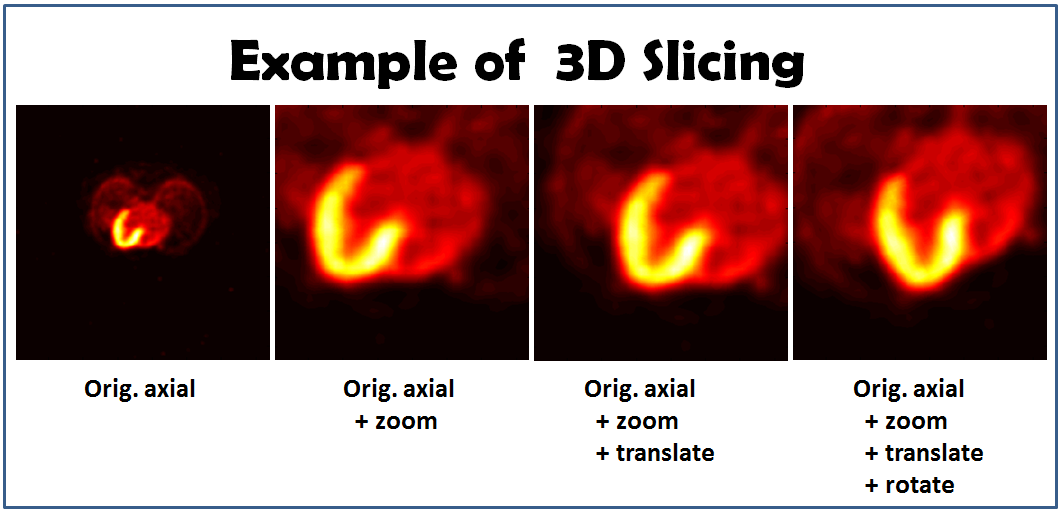
Show the new slice (the new image can be seen the first image in the figure).

  figure, imagesc(slice), axis image, colormap(hot) % show org image

Zooming

We're going to use the approach II to zoom-in the slice in a factor of three.

Set the zoom factor.

  zoomFactor = 3;  % set zoom factor

Calculate the new pixel size.

  pixelSpacing = pixelSpacingOrg / zoomFactor;  % adjust pixel size

After zooming you may need to translate the image center, or you may see nothing.

  originalFOV = [Nc; Nr] .* pixelSpacingOrg;  % calculate the original FOV (mm)
  zoomShift = originalFOV / 2 * (zoomFactor - 1) / zoomFactor ;
  planePos = planePosOrg + [zoomShift ; 0] ;

Generate new slice using coordinateGen() and sliceVolume().

  [u, v, w] = coordinateGen(ivd, Nc, Nr, pixelSpacing, planePos, orientationInput);
  
  slice = sliceVolume(ivd, v , u , w, rawBackgroundPixelValue,'linear');

Show the new slice.

  figure, imagesc(slice), axis image, colormap(hot) % show org +zoom

The new slice is the second image in the figure. It required fewer lines when coding using the approach II.

Translation

Let's try to do the translation using the approach II.

First of all, set the translation matrix.

  transMat = [-35.0; -5; 0];  % the translation in x, y, and z directions

Apply the translation matrix to obtain new plane position.

  planePosTrans = planePos + transMat;

Generate new slice.

  [u, v, w] = coordinateGen(ivd, Nc, Nr, pixelSpacing, planePosTrans, orientationInput);
  
  slice = sliceVolume(ivd, v , u , w, rawBackgroundPixelValue,'linear');

Show the new slice.

  figure, imagesc(slice), axis image, colormap(hot) % show org +zoom+translation

The third picture in the figure is the result of the new slice.

Rotation

In this example, we're going to rotate the original image (counter-clockwise).

Set the angle we want to rotate.

  rotAngle = 25/180*pi;   % rotate 25 degree

Firstly, we create the rotation matrix. You can find more detail about the rotation matrix in [2]. Let's try to rotate the image counter-clockwisely about z-axis.

  rotMat= [ cos(rotAngle), -sin(rotAngle),       0 ;
                  sin(rotAngle),  cos(rotAngle),       0 ;
                                    0,                     0,       1 ];

By combining the rotation matrix and the original orientation marix, we will get a new orientation matrix with rotation.

  orientationInputRot = rotMat * orientationInput;

After rotation, we adjust the center of the rotated image.

  newFOV = [Nc; Nr] .* pixelSpacing;
  transMat2 = orientationInputRot([1, 2], [1,2]) * ( newFOV / 2 ) - newFOV / 2;  % calculate the translation of the original center after rotation
  planePosTrans2 = planePosTrans - [transMat2 ; 0];  % backward translating the rotated image center