Support:Documents:Examples:Model Corrected Input Function

Model-Corrected Input Function

Overview

For ¹⁸F-FDG PET studies, the estimation of kinetic rate constants required knowledge of the input function (i.e., ¹⁸F-FDG plasma time activity curve). The standard method to determine the input function is to measure 18F-FDG activity concentration in the arterial blood. However, this invasive procedure is limited by the small size of blood vessels and the limited blood volume. One alternative way is to estimate the input function non-invasively. One of non-invasive methods is image-derived input functions (IDIFs), which estimate input function from a region of interest (ROI) within the ventricular cavity. However, due to the limited spatial resolution and the cardiac and respiratory motion, cross-contamination from surrounding tissues to vascular structures affects the accuracy of estimated input function. To solve these problems, Fang proposed a model-corrected input function (MCIF), which used simultaneous estimation to correct the spillover and partial volume effect for IDIFs.

Example of Estimating Input Function Using MCIF

Here is an example of COMKAT GUI for estimating kinetic rate constants, and the MCIF method is used to estimate input function.

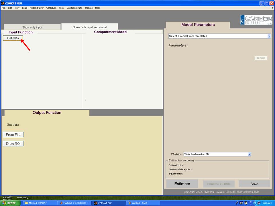
Step 1. Type "comkat" in Matlab commandwindow and "COMKAT_GUI" GUI (below figure) should be started.

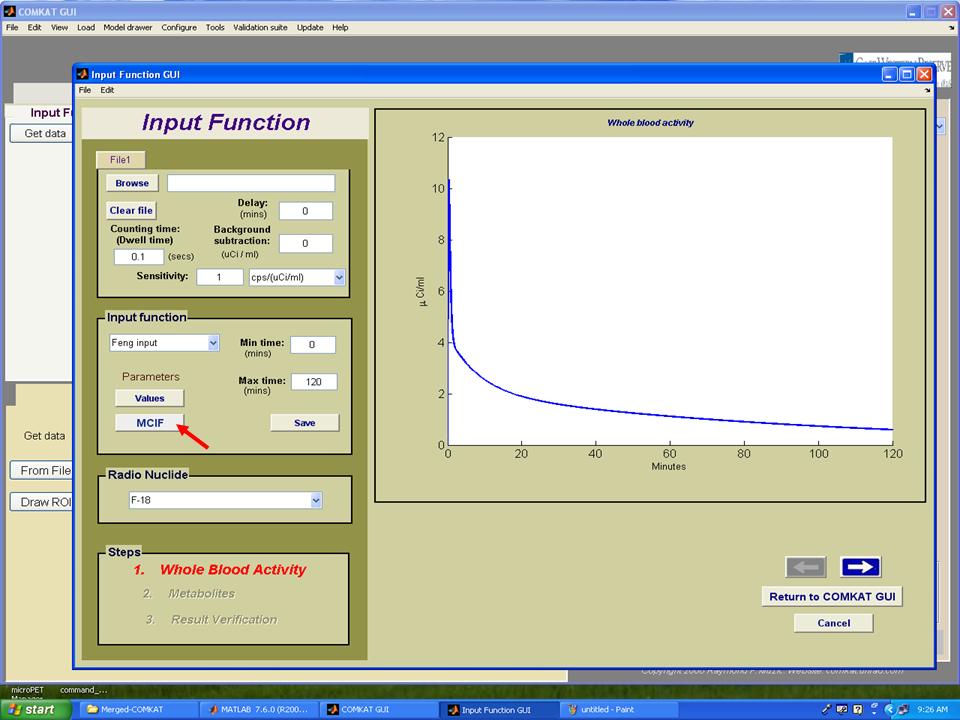
Step 2. Hit 'Get data' button in "COMKAT_GUI" and "Input Function GUI" (below figure) shoud be started.

Step 3. Hit 'MCIF' button in "Input Function GUI" and "inputest" GUI (below figure) shoud be started.

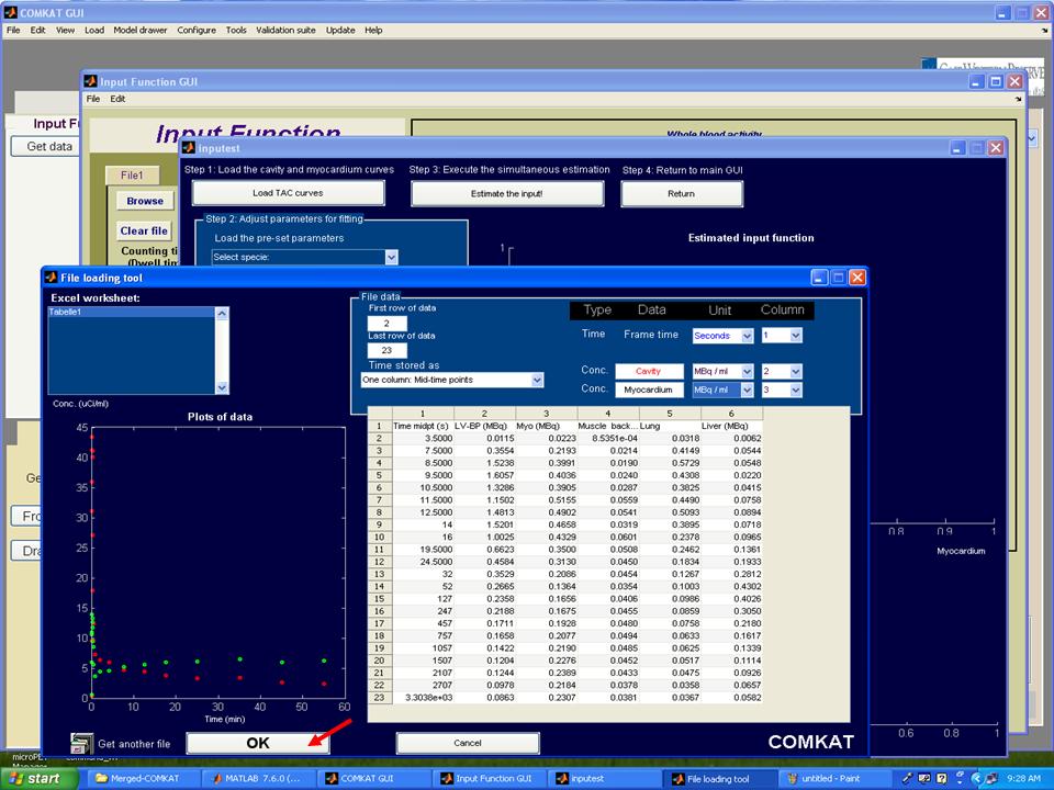
Step 4. Hit 'Load TAC curves' button in "inputest" GUI and "File loading tool" GUI (below figure) should be started. Then, choose concentrations of cavity and myocardium from the file user loaded and set units that user defined. Hit 'OK' button to return to "inputest" GUI.

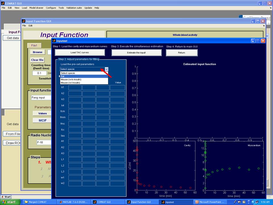
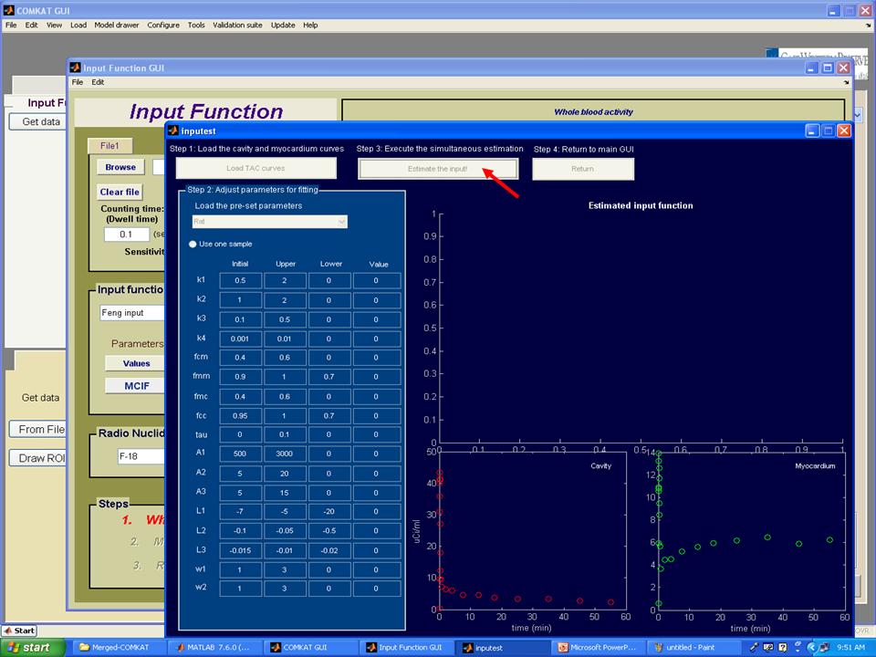
Step 5. Now, the TAC curves for cavity and myocardium should appear in "inputest" GUI (below figure). Then, hit 'Load the pre-set parameters' to choose the animal model user used. Note: pre-set parameters may change with different studies and user should try different initial, upper and lower values.

Step 6. Hit 'Estimate the input' button to start the estimation of parameters. Note: please wait several minutes until the estimation process completed.

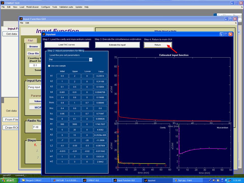
Step 7. As the estimation process completed, the TAC curve for estimated input function should appear in "inputest" GUI (below figure) and the estimated parameters should in the column 'Value'. Then, hit 'Return' button to return to "Input Function GUI".

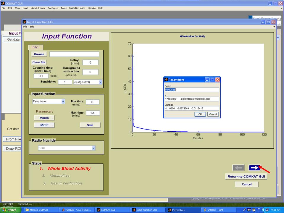
Step 8. The TAC curve for whole blood activity should appear in "Input Function GUI". Note: hit 'Values' to see estimated parameters that define the input function. Hit the arrow to the next step.

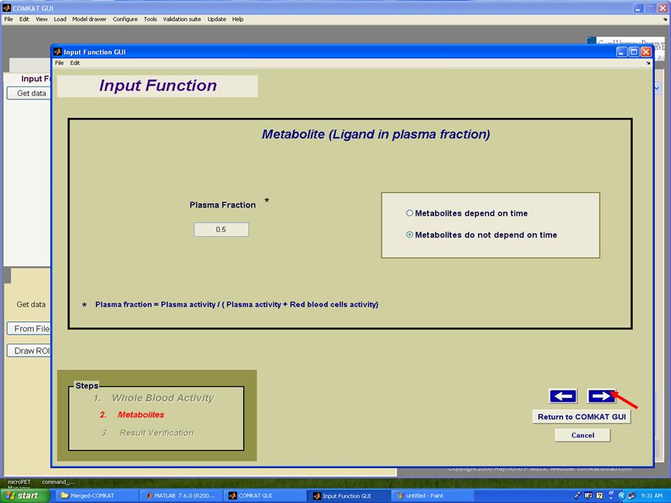
Step 9. Set plasma fraction and then hit the arrow to the next step.

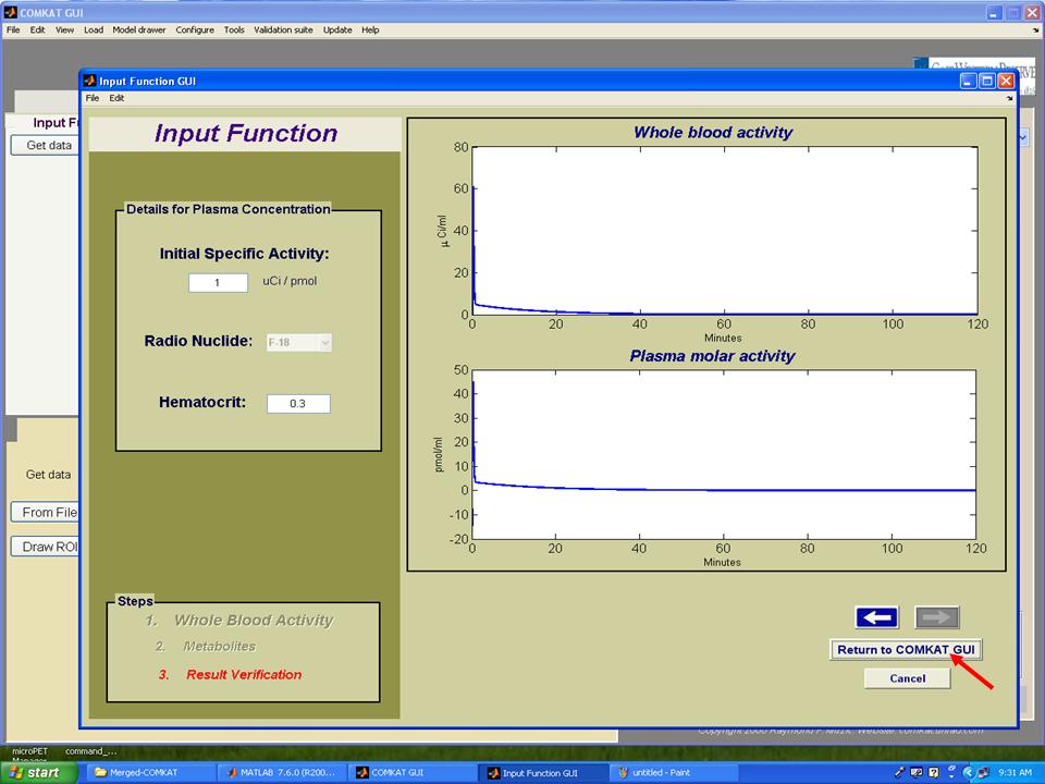
Step 10. Set initial specific activity and hematocrit for producing TAC curve for plasma and then hit 'Return to COMKAT GUI' button to return to "COMKAT GUI".

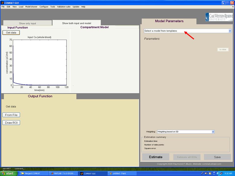
Step 11. The TAC curve for whole blood should appear in "COMKAT GUI" (below figure). Then, hit 'Select a model from templates' button to choose the kinetic model.

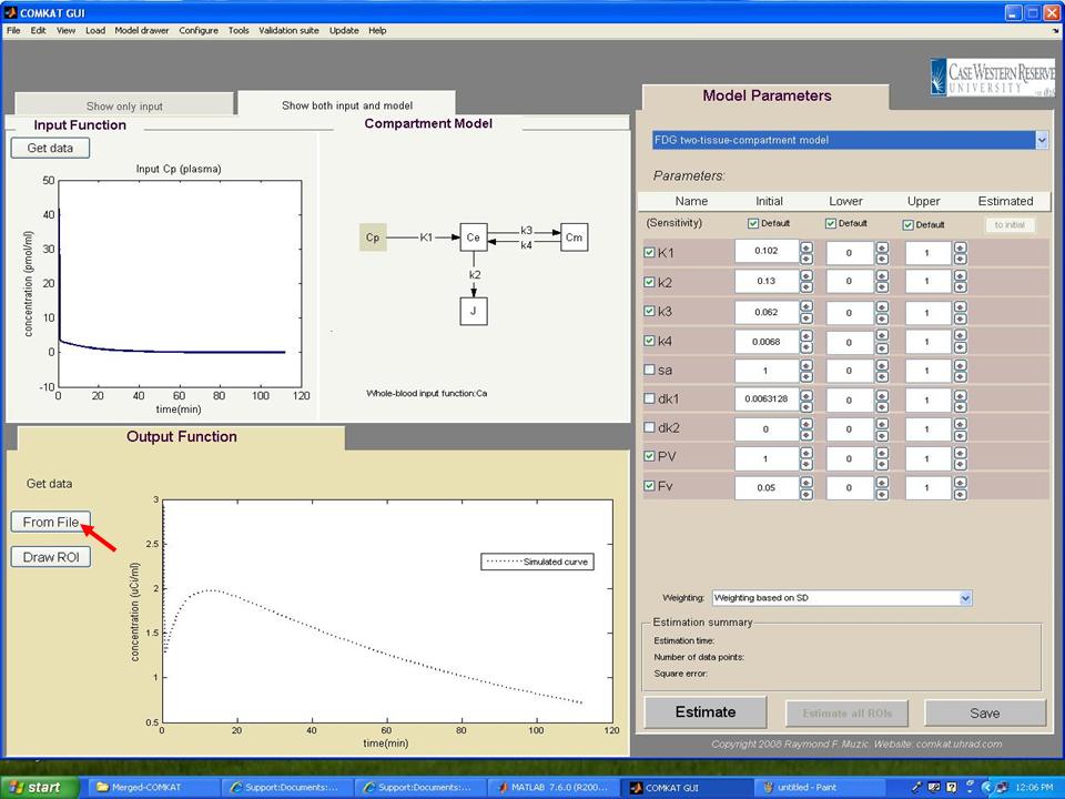
Step 12. In "COMKAT GUI" (below figure), the initial, upper and lower kinetic rate constants for the model should appear in the right side of the figure. Then hit 'From file' or 'Draw ROI' button to load output function.

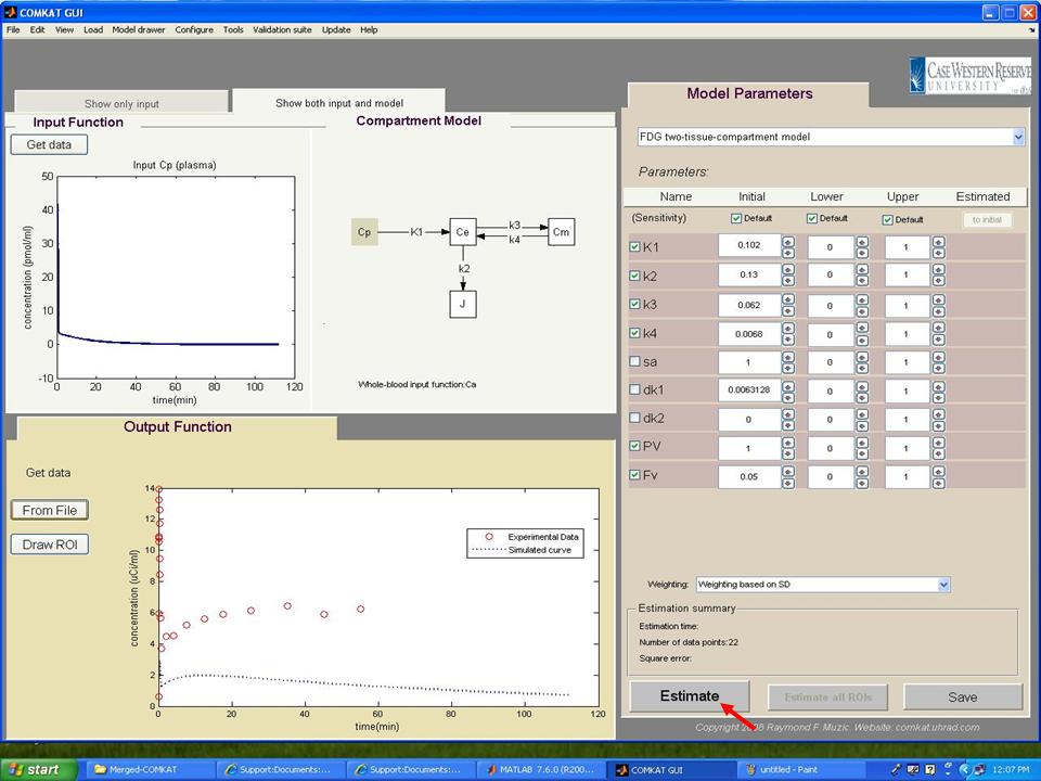
Step 13. After loading output function, the TAC curve (Experimental Data: red circle) should appear in "COMKAT GUI" (below figure). Then, hit 'Estimate' button to start the estimation of parameters.

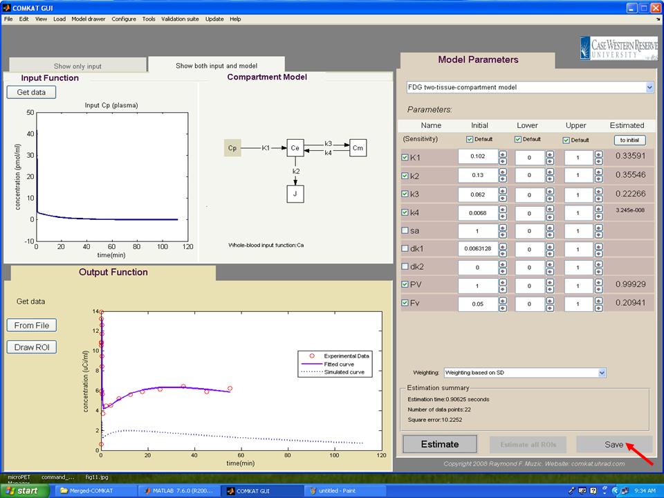
Step 14. After the estimation process, the TAC curve (Fitting Curve: blue line) should appear in "COMKAT GUI" (below figure) and estimated parameters are in the right side of the figure. Then, hit 'Save' button to save results.

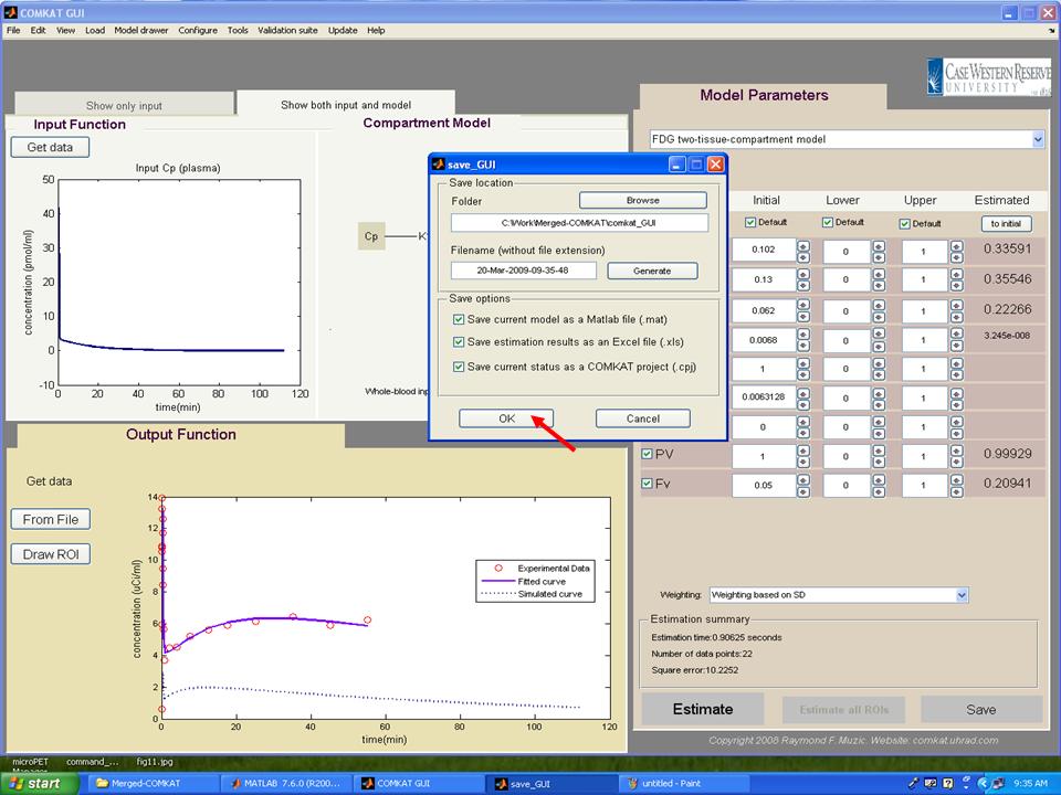
Step 15. In "save_GUI", user can save results as a Matlab file, an Excel file or a COMKAT project in the folder. More details about COMKAT GUI can be found in this document.