Difference between revisions of "Support:Documents:Examples:Estimate Change of Neurotransmitter"
| Line 115: | Line 115: | ||
[[Image:Input2.jpg]] | [[Image:Input2.jpg]] | ||
| + | |||
| + | The endogenous input function is implemented as: | ||
| + | |||
| + | <pre> | ||
| + | function [y, grad] = gammavariate(p,t) | ||
| + | % parameters [p(1) p(2) p(3) p(4) p(5)] = [Basal G alpha beta delay] | ||
| + | y = p(1).*ones(size(t)); | ||
| + | idx = find(t >= p(5)); | ||
| + | dt = t(idx) - p(5); | ||
| + | |||
| + | y(idx) = p(1) + p(2)*(dt.^p(3)).*exp(-p(4).*dt); | ||
| + | |||
| + | if nargout > 1, | ||
| + | grad = zeros(length(t), 5); | ||
| + | grad(:,1)=ones(size(t)); | ||
| + | |||
| + | if ~isempty(idx), | ||
| + | grad(idx,2) = (dt).^p(3).*exp(-p(4).*(dt)); | ||
| + | grad(idx,3) = p(2).*(dt).^p(3).*log(dt).*exp(-p(4).*(dt)); | ||
| + | grad(idx,4) = -p(2).*(dt).^(p(3)+1).*exp(-p(4).*(dt)); | ||
| + | grad(idx,5) = -p(2)*p(3)*(dt).^(p(3)-1).*exp(-p(4).*(dt)) + p(2)*p(4)*(dt).^p(3).*exp(-p(4).*(dt)); %dy/ddelay | ||
| + | end | ||
| + | end | ||
| + | return | ||
| + | </pre> | ||
Revision as of 20:54, 2 March 2009
Model of Neurotransmitter PET (ntPET)
Overview
The changes of endogenous neurotransmitter by PET scanning after a stimulus have been proved with different approaches. In stead of detecting the increase or decrease of a neurotransmitter, it is important to characterize the temporal change of a neurotransmitter after a stimulus. Morris proposed the new technique (called ntPET) for capturing the dynamic changes of a neurotransmitter after a stimulus and demonstrated the ability of this method to reconstruct the temporal characteristics of an enhance in neurotransmitter concentration.
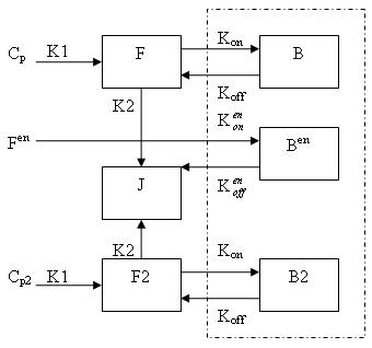
Generally, there are two separate injections of tracer for ntPET: one for the rest condition (without any stimuli) and the other for the activation condition (after a stimulus). Therefore, the model can be described as:
This model can be described by the differential equations:
dF/dt = K1Cp - K2F - Kon[Bmax - B - B2 - Ben]F + koffB
dB/dt = Kon[Bmax - B - B2 - Ben]F - koffB
dF2/dt = K1Cp2 - K2F2 - Kon[Bmax - B - B2 - Ben]F2 + koffB2
dB2/dt = Kon[Bmax - B - B2 - Ben]F2 - koffB2
dBen/dt = Kenon[Bmax - B - B2 - Ben]Fen -kenoffBen
Cp is the plasma concentration of tracer at the first injection (the "rest" condition).
F and B are free (unbound) and bound molar concentrations of tracer after the first injection
Cp2 is the plasma concentration of tracer at the second injection (the "activation" condition).
F2 and B2 are free (unbound) and bound molar concentrations of tracer after the second injection.
Fen and Ben are free and bound molar concentrations of a neurotransmitter released by endogenous ligand after a stimulus.
Bmax is the maximum number of receptors that can be bound by neurotransmitter or tracer.
Bmax - B - B2 - Ben is the concentration of available receptors. This also indicates that binding is saturable.
K1, K2, Kon, Koff, Kenon and Kenoff are rate constants.
Implementing the Compartment Model
Create a new model for ntPET
   %MODEL CONSTRUCTION
    cm = compartmentModel;
   % Set scan time
    inj2Delay = 240; % min between 1st and 2nd inj
    disp('Define one long study: inj 1 = baseline, inj 2 = activation');
    scantInj1 = [[0:0.1:0.9 1:0.25:1.75 2:0.5:4.5 5:1:59]' [0.1:0.1:1 1.25:0.25:2 2.5:0.5:5 6:1:60]'];
    scantInj2 = scantInj1 + inj2Delay;
    scant = [scantInj1; scantInj2];
    deltaT = scant(:,2) - scant(:,1);
    tmid   = 0.5*(scant(:,1) + scant(:,2));
    %Set parameters of the model
    cm = addParameter(cm, 'PV', 1 );
    cm = addParameter(cm, 'Fv', 0);
    cm = addParameter(cm, 'sa', 1);    % uCi/pmol
    cm = addParameter(cm, 'dk', 0);    % assume data are decay-corrected
    cm = addParameter(cm, 'k1',      0.9);
    cm = addParameter(cm, 'k2',      0.4);
    cm = addParameter(cm, 'kon' ,   0.01);
    cm = addParameter(cm, 'koff',    0.14);
    cm = addParameter(cm, 'k2ref',  0.3);
    cm = addParameter(cm, 'Bmax',  80);
    cm = addParameter(cm, 'konEN', 0.25);
    cm = addParameter(cm, 'koffEN', 25);
    %model for baseline condition:
    cm = addCompartment(cm, 'F');
    cm = addCompartment(cm, 'B',      'Bmax');
    cm = addCompartment(cm, 'Junk');

    %model for activation condition:
    cm = addCompartment(cm, 'F2');
    cm = addCompartment(cm, 'B2',      'Bmax');
    cm = addCompartment(cm, 'B^{EN}', 'Bmax');
    % Create input functions for two injections
    t = 0:0.05:305; % coverage out to 6+ h
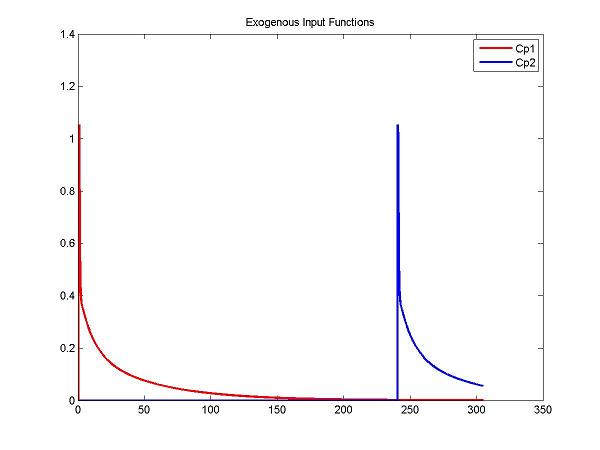
    Cp1Data = fengInput([2 0.5 8.5 0.22 0.2 -4. -0.1 -0.02], t);
    Cp2Data = fengInput([2 inj2Delay+0.5 8.5 0.22 0.2 -4. -0.1 -0.02], t);
    ppCp1 = spline(t, Cp1Data);
    ppCp2 = spline(t, Cp2Data);

    figure; plot(t, ppval(ppCp1, t), 'r', t, ppval(ppCp2,t), 'b', 'LineWidth', 2); title('Exogenous Input Functions'); legend('Cp1', 'Cp2')

    cm = addInput(cm, 'C_p', 'sa', 'dk', 'ppval', ppCp1);
    cm = addInput(cm, 'C_p2', 'sa', 'dk', 'ppval', ppCp2);
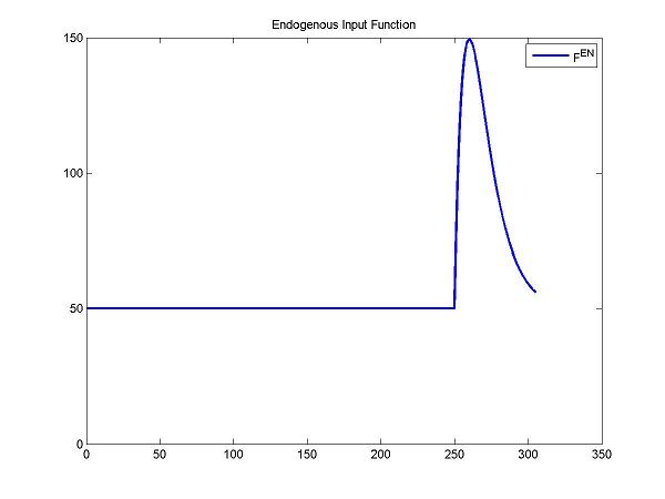
Here, we simulate the endogenous input function (after a stimulus) by a gamma variate function. Fen = Basal + Gamma[t-Delay]Alpha exp(-Beta[t-Delay]). Note: Basal is the concentration of the endogenous neurotransmitter without any stimulus. Gamma, Alpha and Beta control the change of concentrations of the endogenous neurotransmitter. Delay is the delay time.
    DApar = [50 27 1 0.1 240+10]; % = [Basal Gamma Alpha Beta Delay]
    cm = addParameter(cm, 'DA', DApar);
    cm = addInput(cm, 'F^{EN}', 0, 0, 'gammavariate', 'DA'); %DA defined by gamma variate function at activation condition
    figure; plot(t, gamma(DApar, t), 'b', 'LineWidth', 2); title('Endogenous Input Function'); legend('F^{en}');
    ax = axis; axis([ax(1) ax(2) 0 ax(4)]); % ensure minimum y-axis value is zero
The endogenous input function is implemented as:
function [y, grad] = gammavariate(p,t)
% parameters [p(1) p(2) p(3) p(4) p(5)] = [Basal G alpha beta delay]
    y = p(1).*ones(size(t));
    idx = find(t >= p(5));
    dt  = t(idx) - p(5);

    y(idx) = p(1) + p(2)*(dt.^p(3)).*exp(-p(4).*dt);

    if nargout > 1,
        grad = zeros(length(t), 5);
        grad(:,1)=ones(size(t));

        if ~isempty(idx),
            grad(idx,2) = (dt).^p(3).*exp(-p(4).*(dt));
            grad(idx,3) = p(2).*(dt).^p(3).*log(dt).*exp(-p(4).*(dt));
            grad(idx,4) = -p(2).*(dt).^(p(3)+1).*exp(-p(4).*(dt));
            grad(idx,5) = -p(2)*p(3)*(dt).^(p(3)-1).*exp(-p(4).*(dt)) + p(2)*p(4)*(dt).^p(3).*exp(-p(4).*(dt)); %dy/ddelay
        end
    end
return


