Difference between revisions of "Support:Documents:Examples:Estimate Input Parameters Simultaneously with Flow"
| Line 97: | Line 97: | ||
==== Define tissue and blood outputs ==== | ==== Define tissue and blood outputs ==== | ||
| − | Define two model outputs. The output called TissuePixel predicts the activity in a tissue pixel and the output called ArterialPixel predicts the activity that would be observed in a pixel in the aorta. TissuePixel corresponds to C<sub>T</sub>S + F<sub>v</sub>C<sub>a</sub> whereas | + | Define two model outputs. The output called TissuePixel predicts the activity in a tissue pixel and the output called ArterialPixel predicts the activity that would be observed in a pixel in the aorta. TissuePixel corresponds to C<sub>T</sub>S + F<sub>v</sub>C<sub>a</sub> whereas ArterialPixel is 100% C<sub>a</sub>. |
<pre> | <pre> | ||
% define the activity concentration in tissue pixel | % define the activity concentration in tissue pixel | ||
| Line 106: | Line 106: | ||
</pre> | </pre> | ||
| − | Note that COMKAT | + | Note that COMKAT even accounts for the time-averaging of concentrations over the durations of the scan frames. |
| − | + | For simplicity here a sequence of contiguous 10-second frames is used. (Frame start times 0, 10, 20, ... 590 sec and frame end times 10, 20, 30, ... 600 sec). | |
<pre> | <pre> | ||
% specify scan frame times | % specify scan frame times | ||
| − | bfcm = set(bfcm, 'ScanTime', [[0:10:590]' [10:10:600]']/60); | + | bfcm = set(bfcm, 'ScanTime', [[0:10:590]' [10:10:600]']/60); % division by 60 converts sec to min |
</pre> | </pre> | ||
Revision as of 01:28, 8 March 2008
Estimating Input Function Parameters Simultaneously with Flow
This example demonstrates an approach to simultaneously estimating input functions parameters along with blood flow in the context of the PET blood flow model.
Tissue uptake
The flow model has one tissue compartment. Radioactive water (or another freely diffusible molecule) in the blood is assumed to rapidly exchange with that in (extravascular) tissue. The tissue model has two rate constants: K1 and k2 and can be depicted in a diagram:
It can also be described by the differential equation:
dCT/dt = K1 Cp - k2 CT
where CT is the tissue concentration and Cp is the plasma concentration of radioactive water.
CT and Cp are interpreted as either molar concentrations (Salinas 2007).
Instead of estimating K1 and k2, it sometimes is advantageous to estimate a different set of parameters defined as
lambda = K1/k2 and F = K1.
F is blood flow (perfusion) per unit volume of tissue (for simplicity we're assuming 100% extraction) and lambda is the ratio of tissue to blood concentrations at equilibrium.
To use this parameterization in COMKAT, one needs to express the rate constants in terms of lambda and F: K1 = F, k2 = K1/lambda
This example demonstrates how to estimate F (simultaneously with input function parameters). The example could be easily modified to estimate lambda as well.
Input function
This example also demonstrates how to use a parameterized input function. Specifically, the plasma concentration vs. time t is modeled as
Cp = (p1(t-d) - p2 - p3) exp(p4 (t-d)) + p2 exp(p5 (t-d)) + p3 exp(p6(t-d)) [aka Feng input]
d is a time-delay and Cp is defined to be zero for t < d.
In this example, the values of the parameters p1, p2, ... p6 will be estimated.
Note: The Feng input function has been implemented in fin.m in the COMKAT examples folder.
Pixel values
In a PET image, pixel values represent the radioactivity concentration. There are contributions from radioactivity in blood and tissue. The arterial blood concentration includes radioactive water in plasma and the blood cells and is designated Ca. Here we assume Ca can be described using the Feng input equation but with different values for p1, p2, ... p6 than were used for Cp. The tissue activity concentration is CT x S where S is the exponentially-decaying specific activity and CT is given above. The pixel activity concentration is calculated as the activity concentration in the tissue plus the pixel's fractional blood space Fv times the arterial blood activity concentration: PET = CTS + FvCa.
Implement the Compartment Model
Create a new model
First create an new model stored in variable bfcm (blood flow compartment model) and add compartments. The J compartment is not shown in the figure above but is needed to accept the flux from the k2 arrow.
% create new, empty model
bfcm = compartmentModel;

% add compartments
bfcm = addCompartment(bfcm, 'CT');
bfcm = addCompartment(bfcm, 'J');
Specify the input
The specific activity (ratio of activity to molar concentration) is an exponentially decaying function S(t) = S0 exp(-0.341 t) where t is expressed in units of minutes and 0.341 = ln(2)/half-life of 15O and S0 is the specific activity at time t = 0.
% define the initial specific activity and decay constant
sa0 = 1; % specific activity at t=0
dk = 0.341; % O-15 decay constant
Next specify the input functions Cp and Ca for the compartment model. fin is the name of the function that implements Feng input. pCp and pCa are parameter vectors that hold the values of p1, p2, ... p6 for Cp and Ca.
bfcm = addInput(bfcm, 'Cp', sa0, dk, 'fin', 'pCp');
bfcm = addParameter(bfcm, 'pCp', 2*[851.1 21.88 20.81 -4.134 -0.1191 -0.01043 .5]);

bfcm = addInput(bfcm, 'Ca', sa0, dk, 'fin', 'pCa');
bfcm = addParameter(bfcm, 'pCa', [851.1 21.88 20.81 -4.134 -0.1191 -0.01043 .5]);
Define the connections (arrows) between the compartment and input. The link type 'L' indicates linear kinetics from an input to a compartment and type 'K' indicates linear kinetics from one compartment to another.
% connect compartments and inputs
bfcm = addLink(bfcm, 'L', 'Cp', 'CT', 'K1');
bfcm = addLink(bfcm, 'K', 'CT', 'J', 'k2');

% define values for K1, k2 ...
bfcm = addParameter(bfcm, 'K1', 'F');
bfcm = addParameter(bfcm, 'k2', 'K1/lambda');
bfcm = addParameter(bfcm, 'F', 0.5);
bfcm = addParameter(bfcm, 'lambda', 1.0);
bfcm = addParameter(bfcm, 'Fv', 0.05);
Define tissue and blood outputs
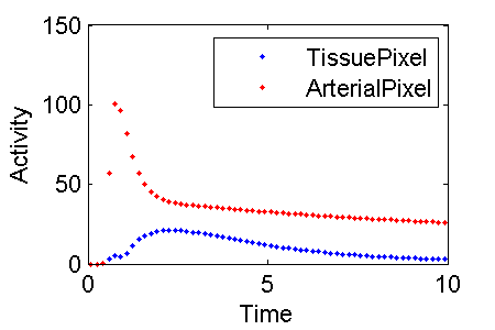
Define two model outputs. The output called TissuePixel predicts the activity in a tissue pixel and the output called ArterialPixel predicts the activity that would be observed in a pixel in the aorta. TissuePixel corresponds to CTS + FvCa whereas ArterialPixel is 100% Ca.
% define the activity concentration in tissue pixel
bfcm = addOutput(bfcm, 'TissuePixel', {'CT', '1'}, {'Ca', 'Fv'});

% define the activity concentration in arterial blood pixel
bfcm = addOutput(bfcm, 'ArterialPixel', {'CT', '0'}, {'Ca', '1'});
Note that COMKAT even accounts for the time-averaging of concentrations over the durations of the scan frames. For simplicity here a sequence of contiguous 10-second frames is used. (Frame start times 0, 10, 20, ... 590 sec and frame end times 10, 20, 30, ... 600 sec).
% specify scan frame times
bfcm = set(bfcm, 'ScanTime', [[0:10:590]' [10:10:600]']/60); % division by 60 converts sec to min
Solve for the model output
Finally, tell COMKAT to solve the model to obtain simulation data that will be used in fitting.
[PET, PETIndex, Output, OutputIndex] = solve(bfcm);

% plot activity in tissue PET(:,3) and blood PET(:,4)
midTime = (PET(:,1) + PET(:,2)) / 2;
plot(midTime, PET(:,3), 'b-', midTime, PET(:,4), 'r.')
legend(PETIndex{3}, PETIndex{4})

% make the figure for this wiki
set(1,'PaperPosition',[0.25 2.5 3 2])
print -dpng c:\temp\ExampleFigureBloodFlowInputModelDataToFit.png
Note, different rows of PET correspond to different frames. The columns of PET hold various quantities as indicated in PETIndex. That is, the contents of column i are described in PETIndex{i}.
Fit Data
Modify the COMKAT model a bit so that it can be used to fit data created above.
Specify the data to fit
Just use the result from above
data = PET(:, [3 4]);
bfcm = set(bfcm, 'ExperimentalData', data);
Specify parameters to estimate along with their initial guesses and range of feasible values.
% specifyparameters to estimate
bfcm = addSensitivity(bfcm, 'pCp', 'F');

% define initial guess and lower and upper bounds
pCpInit = 0.9*2*[851.1 21.88 20.81 -4.134 -0.1191 -0.01043 .5];
FInit = 0.3;
pinit = [pCpInit FInit];
lb = [2*[85 2 2 -8 -3 -0.1 .05] 0.1];
ub = [2*[2000 100 200 -1 -0.01 -0.001 2] 1.];
Note the values of the initial guesses for the input function parameters are 0.9 times the true values. (We're are not cheating by starting with the correct values.)
Do the actual fitting
Fit the data to estimate values of the parameters
[pEst, modelFit] = fit(bfcm, pInit, lb,ub);
COMKAT makes fitting easy!
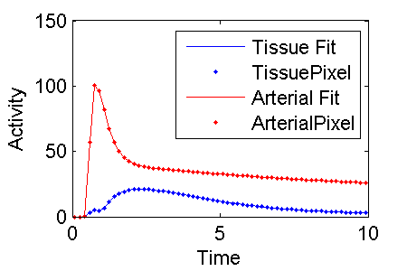
Plot the results and make the figure below for this wiki
plot(midTime, modelFit(:,1), 'b', midTime, PET(:,3), 'b.', midTime, modelFit(:,2), 'r', midTime, PET(:,4), 'r.')
legend('Tissue Fit', PETIndex{3}, 'Arterial Fit', PETIndex{4})
xlabel('Time')
ylabel('Activity')
print -dpng c:\temp\ExampleFigureBloodFlowInputModelFit.png
Ta Da
It looks like a pretty good fit.


