Difference between revisions of "Support:Documents:Examples:Glucose Minimal Model"
Jonihenryser (talk | contribs) m |
|||
| Line 35: | Line 35: | ||
As the glucose minimal model is used to analze blood sample data (and not an image-based data set) for which people usually assume blood samples represent instantaneous (and not the time-averaged) concentration, this example only considers compartment concentrations (and not the output equations). Accordingly, the plots here are based on solutions to the compartment concentrations which are placed in comp when the model is solved using this command: | As the glucose minimal model is used to analze blood sample data (and not an image-based data set) for which people usually assume blood samples represent instantaneous (and not the time-averaged) concentration, this example only considers compartment concentrations (and not the output equations). Accordingly, the plots here are based on solutions to the compartment concentrations which are placed in comp when the model is solved using this command: | ||
| + | |||
| + | [http://vertigosymptoms.co/ Vertigo] | ||
[out, outIndex, comp, compIndex] = solve(cm); | [out, outIndex, comp, compIndex] = solve(cm); | ||
Latest revision as of 22:22, 22 January 2012
This example shows a COMKAT implementation of the glucose minimal model (GMM) which describes the interaction between glucose and insulin in vivo. One model compartment represents interstitial insulin concentration which is denoted by X. Another model compartment represents plasma glucose concentration which is denoted by G. This model was presented in Bergman RN, Ider YZ, Bowden CR, Cobelli C. "Quantitative estimation of insulin sensitivity," Am. J. Physiol., vol. 236, no. 6, pp. E667-E677, June 1979.
Background
Of particular note is that this model has an unusual nonlinear kinetic rule that is different from the nonlinear receptor-ligand and enzyme-substrate kinetic rules. Implementing this GMM in COMKAT required definition of a custom kinetic rule as this example demonstrates. This example also demonstrates COMKAT's ability to solve sensitivity functions (and hence estimate the value of) a parameter which is an initial condition to the differential equations.
Model Equations
dX/dt = -p2 X + p3(I - Ib)
dG/dt = -GX + p1(Gb - G)
with initial conditions X = 0, G = p4 at time zero.
X is interstitial insulin concentration. G is plasma glucose concentration. I is plasma insulin concentration. Ib and Gb are basal insulin and glucose concentrations. p1 to p4 are model mathematical parameters. They are related to the physiologically meaningful parameters as follows
- Glucose effectiveness, SG = p1, a measure of the fractional ability of glucose to enhance its own clearance independent of insulin
- Insulin sensitivity, SI = p3/p2, a measure of the dependence of fractional glucose disposal on changes of plasma insulin
- Initial glucose concentration, G(0) = p4
COMKAT Implementation
To implement the unusual non-linear kinetics present for glucose in COMKAT, the glucose state equation is rearranged to obtain
dG/dt = -G(X + p1) + p1Gb
and the expression (X + p1) is considered as a rate "constant".
Otherwise, the COMKAT implementation is straighforward and the diagram is depicted below.
Model Diagram
Since COMKAT requires a closed system, two junk or sink compartments were created (J1 and J2) so that the efflux from X and G would have a destination.
The complete example is given in comkat\examples\comkatGMM.m.
As the glucose minimal model is used to analze blood sample data (and not an image-based data set) for which people usually assume blood samples represent instantaneous (and not the time-averaged) concentration, this example only considers compartment concentrations (and not the output equations). Accordingly, the plots here are based on solutions to the compartment concentrations which are placed in comp when the model is solved using this command:
Vertigo
[out, outIndex, comp, compIndex] = solve(cm);
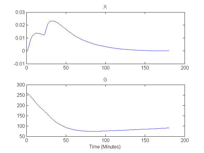
Plots of G and X versus time are shown here:

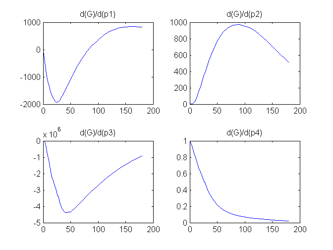
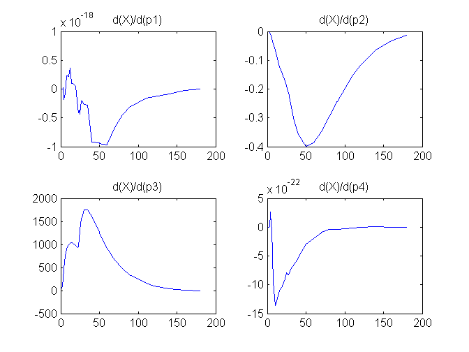
Compartment Concentrations and plots of compartment sensitivity functions, derivatives of X and G with respect to the model parameters, are shown below


Notice that the plots of the sensitivity functions suggest variable X is independent of parameters p1 and p4 as d(X)/d(p1) and d(X)/d(p4) are zero (within the numerical precision). This is expected because a) the state equation for X has neither p1 nor p4 terms and b) G, which appears on the right hand side of the state equation for X, is independent of p1 and p4.
NOTE: GMM is also implemented as part of the validation suite wherein solutions to a COMKAT and an independent implementation are compared.