Difference between revisions of "Support:Documents:Examples:Estimate Change of Neurotransmitter"
| (79 intermediate revisions by 2 users not shown) | |||
| Line 2: | Line 2: | ||
===Overview=== | ===Overview=== | ||
| − | The changes of endogenous neurotransmitter by PET scanning after a stimulus have been proved with different approaches. | + | The changes of endogenous neurotransmitter by PET scanning after a stimulus have been proved with different approaches. Instead of detecting the increase or decrease of a neurotransmitter, it is important to characterize the temporal change of a neurotransmitter after a stimulus. [http://www.ncbi.nlm.nih.gov/pubmed/16285909 Morris (2005)] first proposed the new technique (called ntPET) for capturing the dynamic changes of a neurotransmitter after a stimulus and demonstrated the ability of this method to reconstruct the temporal change in neurotransmitter concentration. More details can be found in following links [[http://www.ncbi.nlm.nih.gov/pubmed/18023364 Normandin 2007], [http://www.ncbi.nlm.nih.gov/pubmed/18296766 Constantinescu 2007], [http://www.ncbi.nlm.nih.gov/pubmed/18176804 Morris 2008], [http://www.ncbi.nlm.nih.gov/pubmed/17354641 Constantinescu 2008]]. |
Generally, there are two separate injections of tracer for ntPET: one for the rest condition (without any stimuli) and the other for the activation condition (after a stimulus). Therefore, the model can be described as: | Generally, there are two separate injections of tracer for ntPET: one for the rest condition (without any stimuli) and the other for the activation condition (after a stimulus). Therefore, the model can be described as: | ||
| Line 8: | Line 8: | ||
[[Image:Model.jpg]] | [[Image:Model.jpg]] | ||
| − | This model can be described by the differential equations: | + | ===Model Equations=== |
| + | |||
| + | This model can be described by the differential equations: | ||
dF/dt = K<sub>1</sub>C<sub>p</sub> - K<sub>2</sub>F - K<sub>on</sub>[B<sub>max</sub> - B - B2 - B<sup>en</sup>]F + k<sub>off</sub>B | dF/dt = K<sub>1</sub>C<sub>p</sub> - K<sub>2</sub>F - K<sub>on</sub>[B<sub>max</sub> - B - B2 - B<sup>en</sup>]F + k<sub>off</sub>B | ||
| Line 35: | Line 37: | ||
F<sup>en</sup> and B<sup>en</sup> are free and bound molar concentrations of a neurotransmitter released by endogenous ligand after a stimulus. | F<sup>en</sup> and B<sup>en</sup> are free and bound molar concentrations of a neurotransmitter released by endogenous ligand after a stimulus. | ||
| − | B<sub>max</sub> is the maximum number of receptors that can be bound by neurotransmitter or | + | B<sub>max</sub> is the maximum number of receptors that can be bound by neurotransmitter or tracer. |
| − | B<sub>max</sub> - B - B2 - B<sup>en</sup> is the concentration of available | + | B<sub>max</sub> - B - B2 - B<sup>en</sup> is the concentration of receptors available for (endogenous and exogenous) ligand binding. This also indicates that binding is saturable. |
| − | K<sub>1</sub>, K<sub>2</sub>, K<sub>on</sub>, K<sub>off</sub>, K<sup>en</sup><sub>on</sub> and | + | K<sub>1</sub>, K<sub>2</sub>, K<sub>on</sub>, K<sub>off</sub>, K<sup>en</sup><sub>on</sub> and K<sup>en</sup><sub>off</sub> are rate constants. |
==Implementing the Compartment Model== | ==Implementing the Compartment Model== | ||
===Create a new model for ntPET=== | ===Create a new model for ntPET=== | ||
| + | |||
| + | Step 1. Create the compartment model | ||
| − | < | + | <pre> |
| − | |||
cm = compartmentModel; | cm = compartmentModel; | ||
| + | |||
| + | %Set scan time of the whole scan | ||
| + | inj2Delay = 240; % min between 1st and 2nd inj | ||
| + | disp('Define one long study: inj 1 = baseline, inj 2 = activation'); | ||
| + | scantInj1 = [[0:0.1:0.9 1:0.25:1.75 2:0.5:4.5 5:1:59]' [0.1:0.1:1 1.25:0.25:2 2.5:0.5:5 6:1:60]']; | ||
| + | scantInj2 = scantInj1 + inj2Delay; | ||
| + | scant = [scantInj1; scantInj2]; | ||
| + | deltaT = scant(:,2) - scant(:,1); | ||
| + | tmid = 0.5*(scant(:,1) + scant(:,2)); | ||
| + | cm = set(cm, 'ScanTime', scant); | ||
| + | |||
| + | %Set parameters of the model | ||
cm = addParameter(cm, 'PV', 1 ); | cm = addParameter(cm, 'PV', 1 ); | ||
cm = addParameter(cm, 'Fv', 0); | cm = addParameter(cm, 'Fv', 0); | ||
cm = addParameter(cm, 'sa', 1); % uCi/pmol | cm = addParameter(cm, 'sa', 1); % uCi/pmol | ||
| − | cm = addParameter(cm, 'dk', 0); % assume data are decay-corrected | + | cm = addParameter(cm, 'dk', 0); % assume data are decay-corrected |
| − | cm = addParameter(cm, ' | + | cm = addParameter(cm, 'k1', 0.9); |
cm = addParameter(cm, 'k2', 0.4); | cm = addParameter(cm, 'k2', 0.4); | ||
cm = addParameter(cm, 'kon' , 0.01); | cm = addParameter(cm, 'kon' , 0.01); | ||
| Line 59: | Line 74: | ||
cm = addParameter(cm, 'Bmax', 80); | cm = addParameter(cm, 'Bmax', 80); | ||
cm = addParameter(cm, 'konEN', 0.25); | cm = addParameter(cm, 'konEN', 0.25); | ||
| − | cm = addParameter(cm, 'koffEN', 25); | + | cm = addParameter(cm, 'koffEN', 25); |
| − | + | ||
%model for baseline condition: | %model for baseline condition: | ||
cm = addCompartment(cm, 'F'); | cm = addCompartment(cm, 'F'); | ||
cm = addCompartment(cm, 'B', 'Bmax'); | cm = addCompartment(cm, 'B', 'Bmax'); | ||
cm = addCompartment(cm, 'Junk'); | cm = addCompartment(cm, 'Junk'); | ||
| − | + | ||
%model for activation condition: | %model for activation condition: | ||
cm = addCompartment(cm, 'F2'); | cm = addCompartment(cm, 'F2'); | ||
cm = addCompartment(cm, 'B2', 'Bmax'); | cm = addCompartment(cm, 'B2', 'Bmax'); | ||
cm = addCompartment(cm, 'B^{EN}', 'Bmax'); | cm = addCompartment(cm, 'B^{EN}', 'Bmax'); | ||
| + | </pre> | ||
| + | |||
| + | Step 2. Set the input function for two injections | ||
| + | |||
| + | <pre> | ||
| + | % Create input functions for two injections | ||
| + | t = 0:0.05:305; % coverage out to 6+ h | ||
| + | Cp1Data = fengInput([2 0.5 8.5 0.22 0.2 -4. -0.1 -0.02], t); | ||
| + | Cp2Data = fengInput([2 inj2Delay+0.5 8.5 0.22 0.2 -4. -0.1 -0.02], t); | ||
| + | ppCp1 = spline(t, Cp1Data); | ||
| + | ppCp2 = spline(t, Cp2Data); | ||
| + | |||
| + | figure; plot(t, ppval(ppCp1, t), 'r', t, ppval(ppCp2,t), 'b', 'LineWidth', 2); title('Exogenous Input Functions'); legend('Cp1', 'Cp2') | ||
| + | |||
| + | cm = addInput(cm, 'C_p', 'sa', 'dk', 'ppval', ppCp1); | ||
| + | cm = addInput(cm, 'C_p2', 'sa', 'dk', 'ppval', ppCp2); | ||
| + | </pre> | ||
| + | |||
| + | [[Image:Input.jpg]] | ||
| + | |||
| + | Step 3. Since the endogenous neurotransmitter is released after a stimulus, we should create an input function that describes the change of concentrations of the endogenous neurotransmitter and estimate the parameters of the function for detecting the change of concentrations of the endogenous neurotransmitter. | ||
| + | |||
| + | The change of concentrations of the endogenous neurotransmitter after a stimulus can be described by a gamma variate function. F<sup>en</sup> = Basal + Gamma[t-Delay]<sup>Alpha</sup> exp(-Beta[t-Delay]). Basal is the concentration of the endogenous neurotransmitter without any stimulus. Gamma, Alpha and Beta control the change of concentrations of the endogenous neurotransmitter. Delay is the delay time. | ||
| + | |||
| + | Note: For ntPET, the initial concentration of the endogenous neurotransmitter (i.e., B<sup>en</sup>) is not zero. At time=0, dB<sup>en</sup>/dt=0 and B=0. Under this condition, B<sup>en</sup>=B<sub>max</sub>F<sup>en</sup>/(k<sup>en</sup><sub>off</sub>/k<sup>en</sup><sub>on</sub>+F<sup>en</sup>). | ||
| + | |||
| + | This indicates that B<sup>en</sup> depends on the F<sup>en</sup>. which is equal to the parameter 'Basal' as time=0. Therefore, during each iteration of solving system models or curve fitting, the initial concentration of the endogenous neurotransmitter at current iteration is dependent on the previous estimated parameter 'Basal'. | ||
| + | |||
| + | To consider this specific case, COMKAT creates a new version of commands for adding parameter. The below command about 'addParameter' is the new version. Instead of using a vector for adding all parameters, we add each parameter as a cell array, individually. This allows COMKAT to track the parameter 'Basal' for calculating the initial concentration of the endogenous neurotransmitter during the solving system models or curve fitting. | ||
| + | |||
| + | This example uses some new features of COMKAT. The version of COMKAT will be soon be made available on the download pages. If you want it sooner, please request it via email. | ||
| + | |||
| + | |||
| + | <pre> | ||
| + | DApar = [50 27 1 0.1 240+10]; % = [Basal Gamma Alpha Beta Delay] | ||
| + | params = {'DAbasal', 'G', 'alpha', 'beta', 'delay'}; | ||
| + | for i = 1:length(params), | ||
| + | cm = addParameter(cm, params{i}, DApar(i)); | ||
| + | end | ||
| + | cm = addInput(cm, 'F^{EN}', 0, 0, 'ntInput', params); | ||
| + | figure; plot(t, ntInput(t,0,params,num2cell(DApar)), 'b', 'LineWidth', 2); title('Endogenous Input Function'); legend('F^{en}'); | ||
| + | cm = addSensitivity(cm, params{:}, 'k1', 'k2', 'kon', 'koff'); | ||
| + | </pre> | ||
| + | |||
| + | [[Image:Input2.jpg]] | ||
| + | |||
| + | The input function of the endogenous neurotransmitter is implemented as (please copy the below function and put in a file called ntInput.m): | ||
| + | |||
| + | <pre> | ||
| + | function [Fen, dFendp] = ntInput(t, nsens, pName, pValue, pSensIdx, cm, xtra) | ||
| + | |||
| + | % This function is used to described endogenous dopamine input. | ||
| + | % The model uses this as | ||
| + | % params = {‘DAbasal’, ‘G’, ‘alpha’, ‘beta’, ‘delay’}; | ||
| + | % cm = addInput(cm, ‘Fen’, 0, 0, ‘ntInput’, params); % don’t need xparameters | ||
| + | % these are not used in this function – only used here to illustrate | ||
| + | % that COMKAT passes the parameter name array. | ||
| + | % The names could be used to generalize this so that it could adapt to | ||
| + | % whatever parameters names and order were specified by the user. | ||
| + | % For simplicity, these are hard-coded for this example. | ||
| + | |||
| + | DAbasalName = pName{1}; | ||
| + | GName = pName{2}; | ||
| + | alphaName = pName{3}; | ||
| + | betaName = pName{4}; | ||
| + | delayName = pName{5}; | ||
| + | |||
| + | % get the values of the named parameters | ||
| + | DAbasal = pValue{1}; | ||
| + | G = pValue {2}; | ||
| + | alpha = pValue{3}; | ||
| + | beta = pValue {4}; | ||
| + | delay = pValue {5}; | ||
| + | |||
| + | if (nargout > 0), | ||
| + | Fen = DAbasal*ones(size(t)); | ||
| + | idx = find(t > delay + 0.001); % offset by 0.001 to avoid numeric instability of the term dt.^(alpha-1) when dt is very near to zero and alpha is less than 1 | ||
| + | dt = t(idx) - delay; | ||
| + | Fen(idx) = DAbasal + G*(dt.^alpha).*exp(-beta.*dt); | ||
| + | |||
| + | if (nargout > 1), | ||
| + | DAbasalSensIdx = pSensIdx{1}; % location (index) of DA among the sensitivity parameters | ||
| + | GSensIdx = pSensIdx{2}; | ||
| + | alphaSensIdx = pSensIdx{3}; | ||
| + | betaSensIdx = pSensIdx{4}; | ||
| + | delaySensIdx = pSensIdx{5}; | ||
| + | |||
| + | % allocate for all sens parameters in model (not just ones relevant to this function) | ||
| + | dFendp = zeros([length(t) nsens]); | ||
| + | dFendp(:, DAbasalSensIdx) = ones(size(t)); % dFen/dDAbasal | ||
| + | if ~isempty(idx), | ||
| + | dFendp(idx, GSensIdx) = dt.^alpha.*exp(-beta.*dt); % dFen/dG | ||
| + | dFendp(idx, alphaSensIdx) = G.*dt.^alpha.*log(dt).*exp(-beta.*dt); % dFen/dalpha | ||
| + | dFendp(idx, betaSensIdx) = -G.*dt.^(alpha+1).*exp(-beta.*dt); % dFen/dbeta | ||
| + | dFendp(idx, delaySensIdx) = -G*alpha.*dt.^(alpha-1).*exp(-beta.*dt) + G*beta.*dt.^alpha.*exp(-beta.*dt); % dFen/ddelay | ||
| + | end | ||
| + | end | ||
| + | end | ||
| + | </pre> | ||
| + | |||
| + | Step 4. Set link between each compartment and add output. | ||
| + | |||
| + | <pre> | ||
| + | %links/output for baseline condition: | ||
| + | cm = addLink(cm, 'L', 'C_p', 'F', 'k1'); | ||
| + | cm = addLink(cm, 'K', 'F', 'Junk', 'k2'); | ||
| + | cm = addLink(cm, 'K2', 'F', 'B', 'kon'); | ||
| + | cm = addLink(cm, 'K', 'B', 'F', 'koff'); | ||
| + | |||
| + | disp('Output is sum of radioactivity in free and bound compartments') | ||
| + | WList = {... | ||
| + | 'F', 'PV'; | ||
| + | 'F2', 'PV'; | ||
| + | 'B', 'PV'; | ||
| + | 'B2', 'PV'}; | ||
| + | XList = {}; | ||
| + | cm = addOutput(cm, 'PET Scan', WList, XList); | ||
| + | |||
| + | %links/output for activation condition: | ||
| + | cm = addLink(cm, 'L', 'C_p2', 'F2', 'k1'); | ||
| + | cm = addLink(cm, 'K', 'F2', 'Junk', 'k2'); | ||
| + | cm = addLink(cm, 'K2', 'F2', 'B2', 'kon'); | ||
| + | cm = addLink(cm, 'L2', 'F^{EN}', 'B^{EN}', 'konEN'); | ||
| + | cm = addLink(cm, 'K', 'B2', 'F2', 'koff'); | ||
| + | cm = addLink(cm, 'K', 'B^{EN}', 'Junk', 'koffEN'); | ||
| + | |||
| + | </pre> | ||
| + | |||
| + | Step 5. Solve the model and generate the output | ||
| + | |||
| + | The new features of setting initial conditions is described below. In order to calculate the initial concentration of the endogenous neurotransmitter (B<sup>en</sup>) at each iteration, we input an equation (declaring as a string) for calculating initial B<sup>en</sup>. This allows COOMKAT to calculate initial B<sup>en</sup> at each iteration. Also, the initial sensitivity of B<sup>en</sup> respect to parameter 'Basal' is determined by this approach. | ||
| + | |||
| + | <pre> | ||
| + | disp('Properly handle the initial conditions assuming no exogenous ligand initially') | ||
| + | compNames = get(cm, 'CompartmentName'); | ||
| + | sensNames = get(cm, 'SensitivityName'); | ||
| + | ncomp = get(cm, 'NumberCompartments'); | ||
| + | idxBENComp = strmatch('B^{EN}', compNames, 'exact'); | ||
| + | idxBasal = strmatch('DA', sensNames); | ||
| + | IC.time = 0; | ||
| + | |||
| + | IC.compartment = cell([ncomp 1]); | ||
| + | IC.compartmentSensitivity = cell([length(compNames) length(sensNames)]); | ||
| + | IC.compartmentSensitivity{idxBENComp, idxBasal} = 'Bmax*(koffEN/konEN) / ((koffEN/konEN + DAbasal)^2)'; | ||
| + | IC.compartment{idxBENComp} = 'Bmax*DAbasal/(koffEN/konEN+DAbasal)'; | ||
| + | cm = set(cm, 'InitialConditions', IC); | ||
| + | |||
| + | [PET, PETIndex, Output, OutputIndex] = solve(cm); | ||
| + | |||
| + | Bmax = pxEval(cm, 'Bmax'); | ||
| + | disp('Plot some compartment concentrations to examine model behavior'); | ||
| + | figure; idx = [3 6]; plot(Output(:,1), Output(:, idx), 'LineWidth', 2); legend(OutputIndex(idx)); title('Free Compartment Concentrations'); | ||
| + | figure; idx = [4 7 8]; plot(Output(:,1), Output(:, idx), [0 Output(end,1)], [Bmax Bmax], 'g:', 'LineWidth', 2); | ||
| + | legend(OutputIndex(idx), 'Bmax'); title('Bound Compartment Concentrations'); | ||
| + | </pre> | ||
| + | |||
| + | For the F compartment, the free molar concentrations of tracer increase after the first injection and then decreases gradually. For the F2 compartment, the free molar concentrations of tracer increase until the secondary injection and then decreases gradually. | ||
| + | |||
| + | At the first injection, the increase of bound molar concentrations of tracer (B) is small due to a lower bounding rate (k1). After a stimulus, the release of neurotransmitters results in an increase of B<sup>en</sup>. The increase of B2 is relatively smaller due to a lower bounding rate (k1). | ||
| + | |||
| + | [[Image:Output1.jpg]] | ||
| + | |||
| + | [[Image:Output2.jpg]] | ||
| + | |||
| + | Step 6. Fit the simulated data | ||
| + | <pre> | ||
| + | % Set upper and lower boundary for each parameter | ||
| + | basal_LB = 30; basal_UB = 70; | ||
| + | gamma_LB = 15; gamma_UB = 50; | ||
| + | alpha_LB = 0.5; alpha_UB = 5; | ||
| + | beta_LB = 0.01; beta_UB = 1; | ||
| + | delay_LB = 240; delay_UB = 300; | ||
| + | k1_LB = 0.01; k1_UB = 3; | ||
| + | k2_LB = 0.01; k2_UB = 1; | ||
| + | kon_LB = 0.001; kon_UB = 0.1; | ||
| + | koff_LB = 0.01; koff_UB = 1; | ||
| + | % Set initial condition for each parameter | ||
| + | pinit = [45 18 1 0.01 250 0.1 0.1 0.005 0.1]; | ||
| + | cm = set(cm, 'ExperimentalData', PET(:,3)); | ||
| + | |||
| + | lb = [basal_LB ; gamma_LB ; alpha_LB ; beta_LB ; delay_LB ; k1_LB ; k2_LB ; kon_LB ; koff_LB]; | ||
| + | ub = [basal_UB ; gamma_UB ; alpha_UB ; beta_UB ; delay_UB ; k1_UB ; k2_UB ; kon_UB ; koff_UB]; | ||
| + | |||
| + | [pfit, modelfit, resnorm, residual, exitFlag, output] = fit(cm, pinit, lb, ub); | ||
| + | |||
| + | figure; plot(t, ntInput(t,0,params,num2cell(DApar)), 'b--',t, ntInput(t,0,params,num2cell(pfit(1:5))), 'r-', 'LineWidth', 1.5); | ||
| + | title('Endogenous Input Function'); legend('True F^{en}','Estimated F^{en}'); | ||
</pre> | </pre> | ||
| + | |||
| + | [[Image:Fitoutput.jpg]] | ||
| + | |||
| + | In the ntPET example, we like to thank Jouni Pesenon for providing useful suggestions. | ||
Latest revision as of 18:22, 30 March 2009
Model of Neurotransmitter PET (ntPET)
Overview
The changes of endogenous neurotransmitter by PET scanning after a stimulus have been proved with different approaches. Instead of detecting the increase or decrease of a neurotransmitter, it is important to characterize the temporal change of a neurotransmitter after a stimulus. Morris (2005) first proposed the new technique (called ntPET) for capturing the dynamic changes of a neurotransmitter after a stimulus and demonstrated the ability of this method to reconstruct the temporal change in neurotransmitter concentration. More details can be found in following links [Normandin 2007, Constantinescu 2007, Morris 2008, Constantinescu 2008].
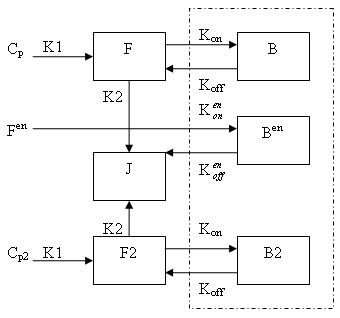
Generally, there are two separate injections of tracer for ntPET: one for the rest condition (without any stimuli) and the other for the activation condition (after a stimulus). Therefore, the model can be described as:
Model Equations
This model can be described by the differential equations:
dF/dt = K1Cp - K2F - Kon[Bmax - B - B2 - Ben]F + koffB
dB/dt = Kon[Bmax - B - B2 - Ben]F - koffB
dF2/dt = K1Cp2 - K2F2 - Kon[Bmax - B - B2 - Ben]F2 + koffB2
dB2/dt = Kon[Bmax - B - B2 - Ben]F2 - koffB2
dBen/dt = Kenon[Bmax - B - B2 - Ben]Fen -kenoffBen
Cp is the plasma concentration of tracer at the first injection (the "rest" condition).
F and B are free (unbound) and bound molar concentrations of tracer after the first injection
Cp2 is the plasma concentration of tracer at the second injection (the "activation" condition).
F2 and B2 are free (unbound) and bound molar concentrations of tracer after the second injection.
Fen and Ben are free and bound molar concentrations of a neurotransmitter released by endogenous ligand after a stimulus.
Bmax is the maximum number of receptors that can be bound by neurotransmitter or tracer.
Bmax - B - B2 - Ben is the concentration of receptors available for (endogenous and exogenous) ligand binding. This also indicates that binding is saturable.
K1, K2, Kon, Koff, Kenon and Kenoff are rate constants.
Implementing the Compartment Model
Create a new model for ntPET
Step 1. Create the compartment model
    cm = compartmentModel;

    %Set scan time of the whole scan
    inj2Delay = 240; % min between 1st and 2nd inj
    disp('Define one long study: inj 1 = baseline, inj 2 = activation');
    scantInj1 = [[0:0.1:0.9 1:0.25:1.75 2:0.5:4.5 5:1:59]' [0.1:0.1:1 1.25:0.25:2 2.5:0.5:5 6:1:60]'];
    scantInj2 = scantInj1 + inj2Delay;
    scant = [scantInj1; scantInj2];
    deltaT = scant(:,2) - scant(:,1);
    tmid   = 0.5*(scant(:,1) + scant(:,2));
    cm = set(cm, 'ScanTime', scant);

    %Set parameters of the model
    cm = addParameter(cm, 'PV', 1 );
    cm = addParameter(cm, 'Fv', 0);
    cm = addParameter(cm, 'sa', 1);    % uCi/pmol
    cm = addParameter(cm, 'dk', 0);    % assume data are decay-corrected
    cm = addParameter(cm, 'k1',      0.9);
    cm = addParameter(cm, 'k2',      0.4);
    cm = addParameter(cm, 'kon' ,   0.01);
    cm = addParameter(cm, 'koff',    0.14);
    cm = addParameter(cm, 'k2ref',  0.3);
    cm = addParameter(cm, 'Bmax',  80);
    cm = addParameter(cm, 'konEN', 0.25);
    cm = addParameter(cm, 'koffEN', 25);

    %model for baseline condition:
    cm = addCompartment(cm, 'F');
    cm = addCompartment(cm, 'B',      'Bmax');
    cm = addCompartment(cm, 'Junk');

    %model for activation condition:
    cm = addCompartment(cm, 'F2');
    cm = addCompartment(cm, 'B2',      'Bmax');
    cm = addCompartment(cm, 'B^{EN}', 'Bmax');
Step 2. Set the input function for two injections
    % Create input functions for two injections
    t = 0:0.05:305; % coverage out to 6+ h
    Cp1Data = fengInput([2 0.5 8.5 0.22 0.2 -4. -0.1 -0.02], t);
    Cp2Data = fengInput([2 inj2Delay+0.5 8.5 0.22 0.2 -4. -0.1 -0.02], t);
    ppCp1 = spline(t, Cp1Data);
    ppCp2 = spline(t, Cp2Data);

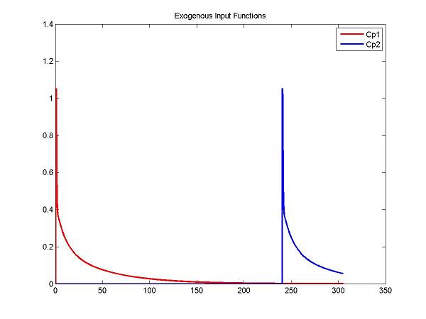
    figure; plot(t, ppval(ppCp1, t), 'r', t, ppval(ppCp2,t), 'b', 'LineWidth', 2); title('Exogenous Input Functions'); legend('Cp1', 'Cp2')

    cm = addInput(cm, 'C_p', 'sa', 'dk', 'ppval', ppCp1);
    cm = addInput(cm, 'C_p2', 'sa', 'dk', 'ppval', ppCp2);
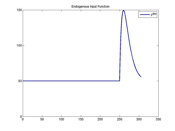
Step 3. Since the endogenous neurotransmitter is released after a stimulus, we should create an input function that describes the change of concentrations of the endogenous neurotransmitter and estimate the parameters of the function for detecting the change of concentrations of the endogenous neurotransmitter.
The change of concentrations of the endogenous neurotransmitter after a stimulus can be described by a gamma variate function. Fen = Basal + Gamma[t-Delay]Alpha exp(-Beta[t-Delay]). Basal is the concentration of the endogenous neurotransmitter without any stimulus. Gamma, Alpha and Beta control the change of concentrations of the endogenous neurotransmitter. Delay is the delay time.
Note: For ntPET, the initial concentration of the endogenous neurotransmitter (i.e., Ben) is not zero. At time=0, dBen/dt=0 and B=0. Under this condition, Ben=BmaxFen/(kenoff/kenon+Fen).
This indicates that Ben depends on the Fen. which is equal to the parameter 'Basal' as time=0. Therefore, during each iteration of solving system models or curve fitting, the initial concentration of the endogenous neurotransmitter at current iteration is dependent on the previous estimated parameter 'Basal'.
To consider this specific case, COMKAT creates a new version of commands for adding parameter. The below command about 'addParameter' is the new version. Instead of using a vector for adding all parameters, we add each parameter as a cell array, individually. This allows COMKAT to track the parameter 'Basal' for calculating the initial concentration of the endogenous neurotransmitter during the solving system models or curve fitting.
This example uses some new features of COMKAT. The version of COMKAT will be soon be made available on the download pages. If you want it sooner, please request it via email.
    DApar = [50 27 1 0.1 240+10]; % = [Basal Gamma Alpha Beta Delay]
    params = {'DAbasal', 'G', 'alpha', 'beta', 'delay'};
    for i = 1:length(params),
        cm = addParameter(cm, params{i}, DApar(i));
    end
    cm = addInput(cm, 'F^{EN}', 0, 0, 'ntInput', params);
    figure; plot(t, ntInput(t,0,params,num2cell(DApar)), 'b', 'LineWidth', 2); title('Endogenous Input Function'); legend('F^{en}');
    cm = addSensitivity(cm, params{:}, 'k1', 'k2', 'kon', 'koff');
The input function of the endogenous neurotransmitter is implemented as (please copy the below function and put in a file called ntInput.m):
function [Fen, dFendp] = ntInput(t, nsens, pName, pValue, pSensIdx, cm, xtra)

% This function is used to described endogenous dopamine input.
% The model uses this as
% params = {‘DAbasal’, ‘G’, ‘alpha’, ‘beta’, ‘delay’};
% cm = addInput(cm, ‘Fen’, 0, 0, ‘ntInput’, params); % don’t need xparameters
% these are not used in this function – only used here to illustrate
% that COMKAT passes the parameter name array.
% The names could be used to generalize this so that it could adapt to
% whatever parameters names and order were specified by the user.
% For simplicity, these are hard-coded for this example.

DAbasalName = pName{1};
GName = pName{2};
alphaName = pName{3};
betaName = pName{4};
delayName = pName{5};

% get the values of the named parameters
DAbasal = pValue{1};
G = pValue {2};
alpha = pValue{3};
beta = pValue {4};
delay = pValue {5};

if (nargout > 0),
    Fen = DAbasal*ones(size(t));
    idx = find(t > delay + 0.001); % offset by 0.001 to avoid numeric instability of the term dt.^(alpha-1) when dt is very near to zero and alpha is less than 1
    dt  = t(idx) - delay;
    Fen(idx) = DAbasal + G*(dt.^alpha).*exp(-beta.*dt);

    if (nargout > 1),
        DAbasalSensIdx = pSensIdx{1}; % location (index) of DA among the sensitivity parameters
        GSensIdx = pSensIdx{2};
        alphaSensIdx = pSensIdx{3};
        betaSensIdx = pSensIdx{4};
        delaySensIdx = pSensIdx{5};

        % allocate for all sens parameters in model (not just ones relevant to this function)
        dFendp = zeros([length(t) nsens]);
        dFendp(:, DAbasalSensIdx) =  ones(size(t)); % dFen/dDAbasal
        if ~isempty(idx),
            dFendp(idx, GSensIdx) =  dt.^alpha.*exp(-beta.*dt); % dFen/dG
            dFendp(idx, alphaSensIdx) =  G.*dt.^alpha.*log(dt).*exp(-beta.*dt); % dFen/dalpha
            dFendp(idx, betaSensIdx) =  -G.*dt.^(alpha+1).*exp(-beta.*dt); % dFen/dbeta
            dFendp(idx, delaySensIdx) =  -G*alpha.*dt.^(alpha-1).*exp(-beta.*dt) + G*beta.*dt.^alpha.*exp(-beta.*dt); % dFen/ddelay
        end
    end
end
Step 4. Set link between each compartment and add output.
    %links/output for baseline condition:
    cm = addLink(cm, 'L',  'C_p',     'F',      'k1');
    cm = addLink(cm, 'K',  'F',       'Junk',   'k2');
    cm = addLink(cm, 'K2', 'F',       'B',      'kon');
    cm = addLink(cm, 'K',  'B',       'F',      'koff');

    disp('Output is sum of radioactivity in free and bound compartments')
    WList = {...
          'F', 'PV';
          'F2', 'PV';
          'B', 'PV';
          'B2', 'PV'};
    XList = {};
    cm = addOutput(cm, 'PET Scan', WList, XList);

    %links/output for activation condition:
    cm = addLink(cm, 'L',  'C_p2',     'F2',      'k1');
    cm = addLink(cm, 'K',  'F2',       'Junk',    'k2');
    cm = addLink(cm, 'K2', 'F2',       'B2',      'kon');
    cm = addLink(cm, 'L2', 'F^{EN}',  'B^{EN}', 'konEN');
    cm = addLink(cm, 'K',  'B2',       'F2',      'koff');
    cm = addLink(cm, 'K',  'B^{EN}',  'Junk',    'koffEN');
Step 5. Solve the model and generate the output
The new features of setting initial conditions is described below. In order to calculate the initial concentration of the endogenous neurotransmitter (Ben) at each iteration, we input an equation (declaring as a string) for calculating initial Ben. This allows COOMKAT to calculate initial Ben at each iteration. Also, the initial sensitivity of Ben respect to parameter 'Basal' is determined by this approach.
    disp('Properly handle the initial conditions assuming no exogenous ligand initially')
    compNames = get(cm, 'CompartmentName');
    sensNames = get(cm, 'SensitivityName');
    ncomp = get(cm, 'NumberCompartments');
    idxBENComp = strmatch('B^{EN}', compNames, 'exact');
    idxBasal = strmatch('DA', sensNames);
    IC.time = 0;

    IC.compartment = cell([ncomp 1]);
    IC.compartmentSensitivity = cell([length(compNames) length(sensNames)]);
    IC.compartmentSensitivity{idxBENComp, idxBasal} = 'Bmax*(koffEN/konEN) / ((koffEN/konEN + DAbasal)^2)';
    IC.compartment{idxBENComp} = 'Bmax*DAbasal/(koffEN/konEN+DAbasal)';
    cm = set(cm, 'InitialConditions', IC);

    [PET, PETIndex, Output, OutputIndex] = solve(cm);

    Bmax = pxEval(cm, 'Bmax');
    disp('Plot some compartment concentrations to examine model behavior');
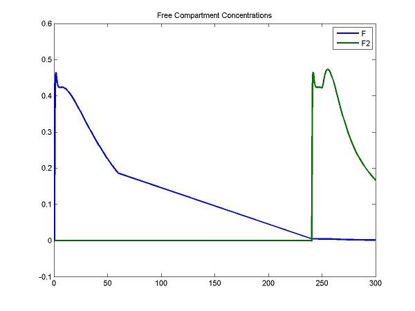
    figure; idx = [3 6]; plot(Output(:,1), Output(:, idx), 'LineWidth', 2); legend(OutputIndex(idx)); title('Free Compartment Concentrations');
    figure; idx = [4 7 8]; plot(Output(:,1), Output(:, idx), [0 Output(end,1)],  [Bmax Bmax], 'g:', 'LineWidth', 2);
    legend(OutputIndex(idx), 'Bmax'); title('Bound   Compartment Concentrations');
For the F compartment, the free molar concentrations of tracer increase after the first injection and then decreases gradually. For the F2 compartment, the free molar concentrations of tracer increase until the secondary injection and then decreases gradually.
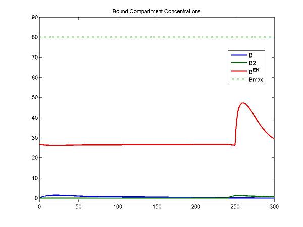
At the first injection, the increase of bound molar concentrations of tracer (B) is small due to a lower bounding rate (k1). After a stimulus, the release of neurotransmitters results in an increase of Ben. The increase of B2 is relatively smaller due to a lower bounding rate (k1).
Step 6. Fit the simulated data
    % Set upper and lower boundary for each parameter
    basal_LB  = 30;      basal_UB  = 70;
    gamma_LB  = 15;      gamma_UB  = 50;
    alpha_LB  = 0.5;    alpha_UB  = 5;
    beta_LB   = 0.01;   beta_UB   = 1;
    delay_LB  = 240;    delay_UB  = 300;
    k1_LB     = 0.01;   k1_UB     = 3;
    k2_LB     = 0.01;   k2_UB     = 1;
    kon_LB    = 0.001;  kon_UB    = 0.1;
    koff_LB   = 0.01;   koff_UB   = 1;
    % Set initial condition for each parameter
    pinit = [45 18 1 0.01 250 0.1 0.1 0.005 0.1];
    cm = set(cm, 'ExperimentalData', PET(:,3));

    lb = [basal_LB ; gamma_LB ; alpha_LB ; beta_LB ; delay_LB ; k1_LB ; k2_LB ; kon_LB ; koff_LB];
    ub = [basal_UB ; gamma_UB ; alpha_UB ; beta_UB ; delay_UB ; k1_UB ; k2_UB ; kon_UB ; koff_UB];

    [pfit, modelfit, resnorm, residual, exitFlag, output] = fit(cm, pinit, lb, ub);

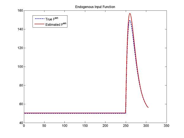
    figure; plot(t, ntInput(t,0,params,num2cell(DApar)), 'b--',t, ntInput(t,0,params,num2cell(pfit(1:5))), 'r-', 'LineWidth', 1.5);
    title('Endogenous Input Function'); legend('True F^{en}','Estimated F^{en}');
In the ntPET example, we like to thank Jouni Pesenon for providing useful suggestions.
