Support:Documents:Examples:Enzyme-substrate (Michaelis-Menten) kinetics

This example demonstrates COMKAT implementation of enzyme substrate (Michaelis Menten) kinetics. This is a type of kinetic rule in which reaction velocity is saturable. As such, this example demonstrates use of a user-specified custom kinetic rule.

Background

Enzymes act as catalysts speeding up reactions wherein a substrate is converted to product without the enzymes themselves being consumed in the process. When the amount of enzyme is much less than the amount of substrate, the effective rate constant k is not actually a constant but rather depends on the substrate concentration

k = Vmax / (Km + [S])

This relationship is described and derived here and requires a couple of approximations.

A COMKAT implementaion of a model that includes such kinetics is given below. The complete model that avoids the two approximations could also be implemented in COMKAT and will be left as an exercise for the student ;-).

COMKAT Implementation

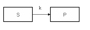
Model figure

This example demonstrates how to implement in COMKAT a model that incorporates the Enzyme-Substrate kinetics using a rate "constant" with a value that depends on substrate concentration. In the interest of simplicity, this example only includes only two compartments and one link. Of course more complicated models could be constructed, yet this example is sufficent to demonstrate the concept.

Step 1 To set this up in MATLAB for simulation, create the following function that defines the rate "constant" for this kinetic rule:

function varargout = kinMM(t, c, ncomp, nsens, pName, pValue, pSensIdx, cm, xtra)
  % Michaelis Menten kinetics
  % flux = C * Vmax/(Km + C) so that effective
  % rate constant k = Vmax/(Km + C)
  VmName = pName{1};
  KmName = pName{2};
  VmValue = pValue{1};
  KmValue = pValue{2};
  VmSensIndex = pSensIdx{1};
  KmSensIndex = pSensIdx{2};
  substrateCompartmentIndex = xtra{1};
  if (nargout > 0), % return effective rate constant
    varargout{1} = VmValue / (KmValue + c(substrateCompartmentIndex));
    if (nargout > 1),  % return dk/dc 
        dkdc = zeros([1 ncomp]); 
        dkdc(substrateCompartmentIndex) = VmValue / (KmValue + c(substrateCompartmentIndex)).^2;
        varargout{2} = dkdc;  
        if (nargout > 2), % return dk/dp
            dkdp = zeros([1 nsens]);
            dkdp(VmSensIndex) = 1 / (KmValue + c(substrateCompartmentIndex));
            dkdp(KmSensIndex) = VmValue / (KmValue + c(substrateCompartmentIndex)).^2;
            varargout{3} = dkdp; % dkdp
        end
    end
  end;
  return;

As for all custom kinetic rules, this function must adhere to the call signature with 8 (or optionally 9) input arguments whether or not all inputs are used. The inputs are

t 	  	    time
c 	  	   Vector of compartment concentrations
ncomp 	       Number of compartments in the model
nsens 	  	Number of parameters for which sensitivity functions are requested (e.g. the number of parameters being estimated_
pName 	      Cell array of character strings. E.g. pName{1} = 'Vm', pName{2} = 'Km'
pValue 	Cell array with pValue{i} being the value of pName{i}
pSensIdx     Cell array containing indicies (locations) of pName{i} in the sensitivityName [addSensitivity()] parameters.
cm 	  	The compartmentModel object
xtra 	  	Any extra information that the user would like to be passed to the function [this input is optional]
 	  	 

The kinMM function is bit complicated because it was written to be general. The compartments that are the source and destination of the link are not hardcoded but rather determined based on the value of the input arguments. Likewise, the names of the parameters that are used to identify what are traditionally described as Km and Vmax are also be specified. Not only does this allow a user call the parameter whatever suits his or her fancy (e.g. the Km value could be specified by a parameter called 'Fred'), it also facilitates models with more than one link that is described by enzyme-substrate kinetics. Writing the function to be general in this fashion obviates having to write a separate kinetic rule function for each model. (The newest verion of the function above is available in comkat\examples\kinMM.m).

One thing to notice about the function above is that the line

varargout{1} = VmValue / (KmValue + c(substrateCompartmentIndex));

corresponds to the equation given in Background.The substrate concentration [S] is taken as the concentration in the source compartment.

Another thing to notice is that the function should return 0, 1 or more values depending nargout. The first return value would be the value of the rate "constant". The second return value would be the derivaive of the rate constant with respect to the concentration vector. The third return value would be the derivative of the rate constant with respect to the sensitivity parameters. These latter two are used in calculating the derivative of model output with respective to sensitivity parameters which is important in data fitting.

Step 2 Create the model.

conc = 10; % initial substrate concentration 

cm = compartmentModel;
cm = addCompartment(cm, 'Substrate');
cm = addCompartment(cm, 'Product');
cm = addParameter(cm, 'Km', 10);
cm = addParameter(cm, 'Vm', 0.5);
cm = addParameter(cm, 'dk', 0); % specific activity
cm = addParameter(cm, 'sa', 1); % decay constant 


% define the time 
tmin = 0;
tmax = 120;
t = [0:1:tmax]';
scanTime = [t t+0.01];
cm = set(cm, 'ScanTime', scanTime); 
 
% details needed for MM kinetics link
substrateCompartmentIndex = { 1 };
pName = {'Vm', 'Km'};           % Vm and Vm parameter names
cm = addLink(cm, 'KSpecial', 'Substrate', 'Product', 'Kmm', 'kinMM', pName, substrateCompartmentIndex); 
 
% set initial concentration and TIME
IC.time = 0;
IC.compartment = [conc; 0];  % all substrate, no product
cm = set(cm, 'InitialConditions', IC); 

% run the model
[cAvg, cAvgIdx, c1, cIdx]  = solve(cm);
 

% repeat experiment with more substrate
IC.compartment = [4*conc; 0];  % all substrate, no product
cm = set(cm, 'InitialConditions', IC);
[cAvg, cAvgIdx, c2, cIdx]  = solve(cm); 

% plot results
plot(c1(:,1), c1(:,[2 3]), c2(:,1), c2(:,[2 3]));
legend('Substrate, Exp 1', 'Product, Exp 1', 'Substrate, Exp 2', 'Product, Exp 2')

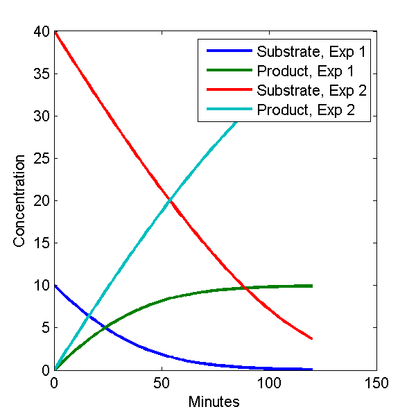
The plot looks like this.

Model Output Plot

A slightly more elaborate version of this example can be found in comkat\examples\tutorialMichaelisMenten.m